While Polymath13 has (barring a mistake that we have not noticed) led to an interesting and clearly publishable result, there are some obvious follow-up questions that we would be wrong not to try to answer before finishing the project, especially as some of them seem to be either essentially solved or promisingly close to a solution. The ones I myself have focused on are the following.
- Is it true that if two random elements
and
of
are chosen, then
for some function
— note that the standard deviation of the sum has order
, so the idea is that this condition should be satisfied one way or the other with probability
).
- Is it true that the stronger conjecture, which is equivalent (given what we now know) to the statement that for almost all pairs
of random dice, the event that
has almost no correlation with the event that
- Can the proof of the result obtained so far be modified to show a similar result for the multisets model?
The status of these three questions, as I see it, is that the first is basically solved — I shall try to justify this claim later in the post, for the second there is a promising approach that will I think lead to a solution — again I shall try to back up this assertion, and while the third feels as though it shouldn’t be impossibly difficult, we have so far made very little progress on it, apart from experimental evidence that suggests that all the results should be similar to those for the balanced sequences model. [Added after finishing the post: I may possibly have made significant progress on the third question as a result of writing this post, but I haven’t checked carefully.]
The strength of a die depends strongly on the sum of its faces.
Let 

is zero, and that the probability that this quantity differs from its average by substantially more than 

As in the proof of the main theorem, it is convenient to define the functions

and
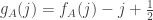
Then

from which it follows that 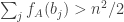

If we choose 


Then 


But


so the expectation of 
By standard probabilistic estimates for sums of independent random variables, with probability at least 


which works out as

Therefore, if 


Why the strong conjecture looks false
As I mentioned, the experimental evidence seems to suggest that the strong conjecture is false. But there is also the outline of an argument that points in the same direction. I’m going to be very sketchy about it, and I don’t expect all the details to be straightforward. (In particular, it looks to me as though the argument will be harder than the argument in the previous section.)
The basic idea comes from a comment of Thomas Budzinski. It is to base a proof on the following structure.
- With probability bounded away from zero, two random dice
- If
Here is how I would imagine going about defining “close”. First of all, note that the function 


If that holds, it should also be the case, since the intervals between 


I’m not quite sure whether proving the second part would require the local central limit theorem in the paper or whether it would be an easier argument that could just use the fact that since 

What about the multisets model?
We haven’t thought about this too hard, but there is a very general approach that looks to me promising. However, it depends on something happening that should be either quite easy to establish or not true, and at the moment I haven’t worked out which, and as far as I know neither has anyone else.
The difficulty is that while we still know in the multisets model that
Of course, we had that difficulty with the balanced-sequences model too, but there we got round the problem by considering purely random sequences
But with the multisets model, there isn’t an obvious way to obtain the distribution over random dice 

A somewhat different approach that I have not got far with myself is to use the standard one-to-one correspondence between increasing sequences of length ![[n]](https://s0.wp.com/latex.php?latex=%5Bn%5D&bg=ffffff&fg=333333&s=0&c=20201002)
![[2n-1]](https://s0.wp.com/latex.php?latex=%5B2n-1%5D&bg=ffffff&fg=333333&s=0&c=20201002)


![S=\{s_1,\dots,s_n\}\subset[2n-1]](https://s0.wp.com/latex.php?latex=S%3D%5C%7Bs_1%2C%5Cdots%2Cs_n%5C%7D%5Csubset%5B2n-1%5D&bg=ffffff&fg=333333&s=0&c=20201002)


Actually, now that I’m writing this, I’m coming to think that I may have accidentally got closer to a solution. The reason is that earlier I was using a holes-and-pegs approach to defining the bijection between multisets and subsets, whereas with this approach, which I had wrongly assumed was essentially the same, there is a nice correspondence between the elements of the multiset and the elements of the set. So I suddenly feel more optimistic that the approach for balanced sequences can be adapted to the multisets model.
I’ll end this post on that optimistic note: no doubt it won’t be long before I run up against some harsh reality.

August 13, 2017 at 2:16 am |
Related to question 3: is it obvious whether or not there exists *any* predicate of dice which is negligible (i.e. ) in the subsets model, but not negligible in the multiset model?
I haven’t been following this project closely, but my impression is that your existing results can be characterized as “all dice behave ‘reasonably’ except for a negligible fraction, and among the ‘reasonable’ ones, our theorems hold, and from this it follows they hold in general”.
So if we take as that predicate that a die is ‘unreasonable’, then if switching to the multiset model (and thus changing the distribution over dice) makes any of the analogous theorem statements false (and if my general understanding is correct), that predicate has to be one which is negligible in the subsets model but not in the multisets model. (Let’s call that a “contrasting predicate”.)
(I’m not conjecturing these “contrasting predicates” don’t exist — in fact, I’m guessing that someone here might be immediately able to give an example of one — maybe it’s enough for the predicate to require that the distribution of element frequencies in the multiset has a certain property. But I’m wondering if thinking about the requirements on such a predicate might be illuminating.)
August 13, 2017 at 2:18 am
(In that comment, I should have defined “negligible” as rather than
  , if there are
  dice of size
  in the model the predicate is about.)
August 13, 2017 at 3:49 am
(A second correction: when I said “subsets model” I should have said “balanced sequences model”.)
August 13, 2017 at 9:20 am
This does seem like a potentially good thing to think about. As you suggest, it probably isn’t hard to come up with distinguishing properties, but it may well be that in some precise sense they are all “irrelevant” to anything one might be interested in when discussing matters such as the probability that one die beats another. (I don’t know how to formulate such a conjecture, but it feels as though something like that might exist.)
If one wants to come up with at least some distinguishing property, it seems good to focus on things like the number of repeated elements, or more generally how the numbers of the different elements are distributed. If we define a map from sequences of length to multisets by writing the sequences in increasing order, then the number of preimages of a multiset depends very strongly on how many repeated elements it has, with extremes ranging from 1 (for the multiset
  ) to
) to  (for the multiset
  ). Since multisets with many repeats give rise to far fewer sequences, one would expect that repeats are favoured in the multisets model compared with the sequences model. I would guess that from this it is possible to come up with some statistic to do with the number of repeats that holds with probability almost 1 in the multisets model and almost zero in the sequences model.
August 13, 2017 at 3:34 pm |
Another possible route to the multi-set result.
Because the random distribution weights between sequence and multiset change so drastically (as you mention it can be as extreme as n! : 1), it feels like either something very special is being exploited for the conjectures to still hold in both models, or this should just happen fairly often with a change of weights. But we’ve already seen that the intransitivity is fairly fragile when changing the dice model.
I think this “something special” is that with the sequences model, not only is the score distribution for a random die very similar to a gaussian, but I conjecture this is true with high probability even when looking at the score distribution for the subset of dice constrained to have some particular multiplicity of values (ie. 12 numbers are unique, 3 are repeated twice, 5 are repeated three times, etc.).
Given the already completed sequence proof, the stricter conjecture is equivalent to saying the U variable is not correlated with the multiplicity of values. Looking at how U is defined, that sounds plausible to me, and may be provable.
If this stricter conjecture is true, then any change of weights for the random distribution will be fine if each “multiplicity class” are changed by the same factor. And this is the case for the shift from sequences -> multiset.
August 13, 2017 at 7:28 pm
That’s a very interesting idea. It seems plausible that as long as a sequence takes enough different values, then conditioning on the distribution of the numbers of times the values are taken shouldn’t affect things too much. It’s not quite so obvious how to prove anything: I don’t see a simple way of using independent random variables and conditioning on an event of not too low probability. But it isn’t obviously impossible, and it would be an interesting generalization if we could get it.
August 14, 2017 at 3:53 am |
> I don’t see a simple way of using independent random variables and conditioning on an event of not too low probability.
(a) I guess the following won’t work, but I’d like to confirm that understanding (and that my reasoning makes sense about the other parts):
If we fix a “multiplicity class”, then a balanced sequence is just a sequence that (1) obeys certain equalities between elements (to make certain subsets of them equal), (2) obeys inequalities between the elements that are supposed to be distinct, (3) has the right sum (so it’s balanced). If the value of each subset of sequence elements which are required equal by (1) is given by an independent random variable, then is the probability of ((2) and (3)) too low? (I guess (2) and (3) are nearly independent.) For (3) I’d guess the probability is similar to the balanced sequence model (the condition still says that some linear sum of the variables has its expected value, I think); for (2) we’re saying that choices of random elements of
 ![[n]](https://s0.wp.com/latex.php?latex=%5Bn%5D&bg=ffffff&fg=333333&s=0&c=20201002) fail to have overlaps, where
fail to have overlaps, where  depends on the multiplicity class but could be nearly as large as
  . I guess the probability of (2) is then roughly exponentially low in
  , which is why this doesn’t work. Is that right?
(b) thinking out loud:
But what if we just omit condition (2)? Then we have some kind of generalization of a “multiplicity class” (except we want to think of it as a random distribution over dice, not just as a class of dice). It’s no longer true that all the dice in this distribution have the same preimage-size in the map from the balanced sequence model to the multiset model… but (in a typical die chosen from this distribution) most of the random variables have no overlaps with other ones, so only a few of the
  subsets of forced-equal sequence elements merge together to increase that preimage size. Can we conclude anything useful from this?
(We would want to first choose and fix one of these distributions, then show that using it to choose dice preserves the desired theorems, then show that choosing the original distribution properly (i.e. according to the right probability for each one) ends up approximating choosing a die using our desired distribution. In other words, we’d want some sum of these sort-of-like-multiplicity-class distributions to approximate our desired overall distribution.)
August 14, 2017 at 8:44 am
Yes, the problem you identify is indeed the problem: I think that typically the multiplicities for a random multiset will have something close to a Poisson distribution with mean 1 (they are given by the lengths of runs of consecutive elements of a random subset of of length
  ). So they will almost all be of constant size, and therefore the number of distinct values taken will be proportional to
  , which implies that the probability that they are distinct is exponentially small.
The difficulty with just not worrying about such coincidences as occur is that the weights are very sensitive to the numbers of coincidences. For example, if two values of multiplicity 3 are allowed to merge into one value of multiplicity 6, then the weight gets divided by . And it seems that to take account of this brings us back to the problem we started with (since if we knew how to deal with these mergers then we could simply take the multiplicity class to be all singletons and deal directly with the multiset model).
That’s just how it seems to me, but as with my previous remarks, anything that sounds pessimistic can potentially be knocked down by some observation that I have not made, or some additional factor that I have not taken into account, and I don’t rule that out here.
August 14, 2017 at 7:27 pm
> And it seems that to take account of this brings us back to the problem we started with …
That’s a good point, and I don’t see a way around it either.
But now I am thinking that “being excluded from the analysis in your main theorem” is *not* uncorrelated with “having lots of repeated faces” (and thus being relatively overrepresented in the multiset model), but is *negatively* correlated with it. If that’s true, then at least in some sense the main theorem should be easier in the multiset model than in the balanced sequence model (since the excluded cases are less common in its distribution).
It’s taking me awhile to write up my reasons for that thought (and even once written they will be vague), so I thought I’d mention that general idea first.
August 14, 2017 at 8:12 pm
One reason that lots of repeated faces make things a bit harder is that it is slightly more complicated to say that the sum has a good chance of equalling a specified value, and probably some of the deviation estimates become worse. But I don’t think those effects would kick in in a serious way until the number of repeats is very large.
August 17, 2017 at 11:08 am |
Here are a few more remarks about the sketch of proof for the (false) strong conjecture. For an unconditioned dice, has the same distribution as a random walk with Poisson(1) steps, conditioned on
  . Hence,
  is a random walk with Poisson(1)-1 steps, conditioned on
  and
and  (I don’t know if it has already been noticed).
Hence, showing that with macroscopic probability, and
and  are close for every
  should not be very hard. For a nonconditioned dice, the variables
  and
and  should be approximately Gaussian with explicit covariances, so for a conditioned dice the
  are still jointly Gaussian. Proving it properly would require a local limit theorem to handle the double conditioning. But this time, the step distribution is known and very simple, so the proof should be easier than the previous one (or, even better, maybe a general result could be applied).
On the other hand, deducing from here that and
and  are uniformly close does not seem obvious. We would need to show that
  cannot vary too much in a short interval. A possible way would be to show that
  is in some sense absolutely continuous with respect to a nonconditioned random walk, and then to use known results about the max of a random walk on a short interval. The absolute continuity also requires a local limit theorem, but this should not be too hard for the same reasons as above.
August 17, 2017 at 9:01 pm |
For the sequence model you can base the criteria if dice A beats dice B on other rules (which can be described e.g. in terms of a function from (-1,1,0)^n to {-1,1,0}). For example dice A beats dice B if the largest “run” of wins of A vs B is larger than the largest runs of wins of B vs A. In analogy with voting rules I would expect that many rules will lead to asymptotic randomness (or pseudoandomness) even when you drop the condition on the sum of entries. (All my previous guesses based on this analogy failed but at least I figured for myself what was the difference.)
August 24, 2017 at 5:38 pm |
Can you delete the previous post? It got mangled because I used less than and greater than characters.
A partial sketch of a different approach.
Consider the starting point: instead of dice represented as a vector of values, represent it as a multiplicity vector m_i = number of faces with value i. A scoring function f(A,B), which gives the number of rolls where A beats B – the number of rolls where B beats A, can be represented as a matrix equation A.F.B where F is an antisymmetric matrix. The constraints are now that m_i ≥ 0, the sum m_i = n, and sum i m_i = n(n+1)/2. The standard die in this representation (1,1,…,1) ties all dice due to theses constraints. Now in the realm of linear algebra, we can choose a set of changes that when starting from a valid die preserves the sum constraints, and that this set of changes spans the valid dice space. I will call this set the choice of dice “steps”. With a given choice of steps, this also provides a distance measurement: the minimum number of steps from the standard die.
With this setup, we can handle both the sequence and multiset dice model if we allow the notion of a “random die” to involve a possibly non-uniform weight on this representation.
Obviously not all weights will lead to intransitive dice. I believe an appropriate restriction would be to constrain possible weights to one such that it is symmetric to permutation of the multiplicity vector in the following way:
– any multiplicity vectors which are the same up to permutation, and meet the sum constraints, will have the same weight
We can choose steps such that the following are true:
– the set of dice one step away from the standard die have the properties:
– 0 ≤ m_i ≤ 2
– each die’s multiplicity vector is the same up to permutation
– each die beats exactly as many dice as it loses to
– all proper dice can be reached in O(n) steps
With such a choice of dice steps, and with the above constraints on the weights under consideration, the set of dice a distance 1 away from the standard die have the property:
– for any die, its probability of beating a random die is exactly equal to its probability of losing to a random die
This is a good starting point, and we can build up to any die by adding these steps together. Furthermore the scoring is linear, so knowing how the steps score against each other is sufficient. With multiple steps, due to correlations it is possible for the set of dice to no longer have every die beat exactly half the others. Since the starting point exactly has this symmetry, if the correlation is small enough combined with the weight constraint restricting the amount of asymmetry that can build up, since all dice can be reached in O(n) steps, maybe the asymmetry can’t build up “fast enough” to ruin the property we want for intransitive dice:
– If A is a random die then with probability 1 – o(1), the probability A beats a random die is equal to the probability it loses to a random die + o(1).
Maybe with a stronger constraint on the weights, one could also show that the probability A beats a random die is 1/2 + o(1), so that it also provides that the ties go to zero. But with such wild swings in the weights between sequence and multiset dice, I’m not sure what would likely be the appropriate strengthening which would also give the ties conjecture.
I believe something like this approach may have been discussed before, but part of the issue with this is the m_i ≥ 0 constraint. It makes it difficult as not all step combinations are valid. However, if the weight constraint above is sufficient, we can temporarily consider them all valid, and it just happens that for sequences and multiset models, the weight for these dice is 0. This approach therefore allows smoothing out the difficulties with considering all the different representations on the same footing, if indeed that weight constraint is sufficient.
Before I think about this approach any further, is there some simple argument or counter-example which shows steps with these properties + weight constraint is not sufficient?
Currently it appears to fit with our understanding:
– sequence dice model is intransitive
– multiset dice model is intransitive
– the improper dice model is mostly transitive (even though it is “balanced” in that every die has the same expectation value, it doesn’t have the nice choice of steps)
– the un-balanced sequence model (sequence model without the sum constraint) is mostly transitive (again, it doesn’t have the nice choice of steps)
– removing the weights constraint we can just choose weights to force transitivity
I’m hoping something along these lines would work as it unites a lot of the results.
August 27, 2017 at 8:04 am |
Another question that’s relevant to statistical theory: it appears that the ordering given by agrees with the ordering based on the sum and hence the mean. Is that true for other reasonable summaries (eg the median, or more generally for some class of linear combinations of order statistics)?
The reason this is interesting is that ordering of distributions based on for *samples* is the (widely-used) Mann-Whitney/Wilcoxon test. It’s already an advance to know this is typically transitive when the means are different, even under just one generating model for distributions. It would be even more helpful to know if this is just a fact about reasonable dice behaving reasonably or something special about the mean.
August 27, 2017 at 9:41 am
I think the mean may be fairly special here. The argument above shows that for two random dice and
and  with means that differ by a typical amount, the means almost certainly determine which one wins. But then another order statistic will not determine which one wins unless it typically agrees with the mean. My guess (though I haven’t thought about it properly, so I may be wrong) is that there is a probability bounded away from zero that the order of the medians of two random sequences is different from the order of the means. If that guess is correct, then the medians will not predict which die wins.
August 28, 2017 at 5:01 am
For dice where the mean is constrained but we allow values greater than n, this also appears to become transitive. In this case the mean is not a predictor, so some other property might give a summary.
Who knows, maybe the median becomes important. I’m not sure anyone has looked into that yet.
August 28, 2017 at 2:16 pm
That’s a great question and something I’d love to see the answer to. Just to clarify the question, when you say “this also appears to become transitive” do you mean that it appears to become transitive with probability or just that there is a positive correlation between the events “A beats B and B beats C” and “A beats C”? If it’s the first, it should be easier to prove, and something I’d either like to have a go at or leave as a tempting open problem in the paper. I’m not sure how to go about analysing the model itself, since it doesn’t seem to be obtainable by some simple conditioning on a sum of independent random variables. On the other hand, I’m pretty sure it (and even more so its continuous counterpart) has been studied a lot, so maybe with a look at the literature we would understand how to prove things about it. Maybe someone reading this can even suggest where to look. (Just to be clear, the distribution I’m interested in is the uniform distribution over the face of the
  -dimensional simplex consisting of all vectors in
  with non-negative coordinates that sum to 1.)
I very much doubt that the median plays an important role here, but if transitivity holds with probability it would be a very nice challenge to try to find a simple statistic that predicts which die will win.
August 28, 2017 at 2:21 pm
Ah, I’ve just looked at the original paper and it does look likely from the evidence presented there that the probability of intransitivity tends to zero for this model (though that was for multisets — it might be interesting to see if the same holds for sequences).
August 31, 2017 at 9:46 pm
I looked into the improper dice (mean still constrained to (n+1)/2, but values are now only constrained to be more than 0).
If you take any proper die and choose an entry greater than 1, and decrease it by one, then compared to the standard die (looking at the possible roll combinations) it will win one less and lose one more. And for any die, if you choose an entry = n, and increase it by one, it will win only one more compared to the standard die. Increasing any value beyond n+1 does not give any added benefit when comparing to the standard die. Therefore, the standard die will beat any improper die with a value greater than n. It beats any “truly” improper die if you will.
From some numerical tests on small sided dice, if we rank all the dice according to how many dice it beats – how many it loses to, the standard die is at the top or at least in the top few dice. At the bottom is the die that is all ones except a single face, as that loses to everything.
Basically, since the “beats” relationship doesn’t care how much a die wins by in a particular roll, deviating from proper dice is only “wasting” pips on a lopsided distribution of value. For this reason, the median does roughly correlate with the order of the improper dice. As does the standard deviation. I would need to look at larger dice to understand the trend better, but I’d guess currently that these will only end up being weak correlations. There is likely a better predictor.
In the proper die scenario the standard die tied everything and was in some sense at the ‘center’ of the dice. In the improper dice, the standard die is now near the top of the ranking, and the die that loses to all other dice is in a reasonable sense the ‘furthest’ from the standard die. So likely there is a measure of ‘distance’ from the standard die that strongly correlates with the ranking (and so strongly predicts if two die beat each other). I think the median would only weakly capture this at best as n gets larger.
If we look at the sequence model of improper dice, what is the probability that at least one value is greater than n? Is it possible that the standard die beats 1 – o(n) fraction of the improper dice?
September 1, 2017 at 3:44 pm
I’ve just realized that the sequence model of improper dice isn’t as hard as I thought. If we line up points with
  gaps between them, then there’s a one-to-one correspondence between sequences of
  numbers that add up to
  , and ways of choosing
  gaps (that mark the point where one number finishes and the next number starts). So the total number of improper dice is
  , which is reasonably close to
  . When the numbers are constrained to be at most
  , then the number of sequences is at most
  , but because the sum of a random sequence has standard deviation about
  , it’s in fact more like
  . A crude estimate of
  is
is  . Since
  , this is exponentially bigger than the number of sequences in the more constrained model. So I think the answer to your last question is yes.
I think we can also say something about the typical shape of an improper die. Suppose that instead of selecting exactly gaps, we select each gap independently with probability
  . The distribution should be similar. But with this model, the expected gap length has a geometrical distribution with mean approximately
  (because
  is about
  ). So it looks to me as though at least crudely speaking an improper die is what you get when you replace the uniform distribution on
 ![[n]](https://s0.wp.com/latex.php?latex=%5Bn%5D&bg=ffffff&fg=333333&s=0&c=20201002) by a geometric distribution with the same mean.
by a geometric distribution with the same mean.
September 2, 2017 at 11:22 pm
I have a guess about a statistic that I think will predict the winner in the sequence model for nonstandard dice. (That is, a random die is a random sequence of positive integers that add up to .)
.)
Let , let
, let  , and for each positive integer
  , let
, let  be the probability of choosing
  with the geometric distribution with parameter
  : that is,
  . (This is sometimes called the shifted geometric distribution.)
In the usual sequence model, the sum of a sequence can be equivalently defined as the number of pairs
  such that
  , which is closely related to how well the die does when it is up against the standard die. And this sum is the right statistic to choose. Note that a random face of the standard die is uniformly distributed in
 ![[n]](https://s0.wp.com/latex.php?latex=%5Bn%5D&bg=ffffff&fg=333333&s=0&c=20201002) .
.
After the heuristic idea in my previous comment, it seems a rather plausible guess that the right statistic to choose for nonstandard dice is how well a die does against not the uniform distribution but the geometric distribution. So that statistic I propose is
Another way of thinking of this is that the sum of a sequence is (up to a factor
  ) the sum of the values of the cumulative distribution function at the numbers
  , where the distribution is uniform on
 ![[n]](https://s0.wp.com/latex.php?latex=%5Bn%5D&bg=ffffff&fg=333333&s=0&c=20201002) . Now I want to take the sum of the values of the cumulative distribution function of the geometric distribution.
. Now I want to take the sum of the values of the cumulative distribution function of the geometric distribution.
Since generating a random improper die is easy, it should be easy to test this hypothesis experimentally. If it checks out, then I’ll sit down and try to prove it.
September 3, 2017 at 9:24 am
Of course, the natural follow-up question if the conjecture in my previous comment is correct is whether if we condition on the improper dice taking the expected value for that statistic we get intransitivity with probability 1/4+o(1) again. If that turned out to be the case, then it would probably be a special case of a much more general principle, which would say that the following picture holds for a wide class of models.
1. For each positive integer , let
, let  be the probability that a given face of a random die from the model takes the value
  . Let
. Let  be the cumulative distribution: that is,
  , which is the probability that the face takes value at most
  .
.
2. Given a die , define
  to be
to be  . Then, with probability
  ,
,  beats
beats  if and only if
  .
.
3. If we fix a value and restrict attention to dice
  for which
  (subject to some condition that ensures that the proportion of dice that satisfy this condition is not too small — for some models we might have to replace the condition by
  ), then the probability that a random triple of dice is transitive is 1/4+o(1).
If we could prove something like this, it would be a significant step forward in our understanding of the intransitivity phenomenon.
Having said that, there is also a suggestion in the paper that for at least one model we get intermediate behaviour, where knowing that beats
beats  and
and  beats
beats  makes it more likely that
  beats
beats  , but with conditional probability bounded away from 1. The model in question is where you choose
  values independently and uniformly from
 ![[0,1]](https://s0.wp.com/latex.php?latex=%5B0%2C1%5D&bg=ffffff&fg=333333&s=0&c=20201002) and then rescale so that the average becomes
and then rescale so that the average becomes  . For a full understanding, it would be good to understand this too.
September 3, 2017 at 10:32 am
Following on from the last paragraph of the previous comment, I now think it would be very nice to get a heuristic understanding (at least) of that rescaled-uniform model. A natural question is the following. Let be a random die chosen according to that model. Let
  be the average value of
  before the rescaling. Does
  correlate with the proportion of dice beaten by
  ?
?
We might expect the answer to be yes for the following reason: if is less than 1/2, then after rescaling, the values below 1/2 are slightly “squashed”, whereas the values above 1/2 are slightly “stretched”. But as P. Peng suggests above, a face does not get extra credit for beating another face by a large margin, so in some sense large values are a “waste of resources”. So one might expect (but this argument is so vague as not to be very reliable) at least a weak positive correlation between
  and the strength of the die. This is something else that would be interesting to test experimentally.
The dream for this model would still be to find a simple statistic that predicts which die wins. Such a statistic couldn’t take values in a totally ordered set (so some simple one-dimensional parameter wouldn’t do, for example), because that would imply transitivity with probability 1-o(1), which seems not to apply. But one could still hope for a map that takes each die to a point in some tournament with a very simple structure, in such a way that the direction of the edge between
  and
and  predicts which of
  and
and  wins. And then the problem would be reduced to understanding the tournament.
Come to think of it, that dream is one that could also be entertained for the balanced sequence model. We know that transitivity occurs with the frequency one gets in a random tournament, but we suspect that the tournament is not quasirandom. These two statements are consistent, because all we need for the transitivity statement is that almost all vertices have roughly the same out-degree as in-degree. So now we can ask what the structure of the tournament is like? Perhaps once you condition on the sum of the faces, there is some other statistic — again, I would hope for a tournament with a nice simple structure — that predicts with high accuracy which of two dice will win.
I don’t yet have a good definition of “nice simple structure”, but an example of the kind of thing I mean is a circle where there is an arrow from to
to  if
if  is less than half way round in a clockwise direction from
  and from
  to
to  if
if  is more than half way round. (If
  is exactly half way round, then the direction of the arrow is chosen arbitrarily.) It is unlikely that we can associate with each die in the balanced-sequence model a point in the circle in such a way that this particular tournament predicts which die wins, but perhaps some higher-dimensional (but still low-dimensional) variant works. If we could do something like this, then we would have a wonderfully precise understanding of the Mann-Whitney/Wilcoxon test for this model.
September 4, 2017 at 3:01 pm |
I’ve thought a bit about the “dream” in this comment from the previous thread, and while I now feel somewhat less optimistic about it, I now have a new (to me anyway) way of thinking about the “beats” relation that I think has the potential to be helpful, and to capture the idea of “wasting resources” by winning too well for no extra reward.
An initial thought is that if A and B are typical dice, then and
and  grow approximately like
  , so unless
  and
and  are close (which usually means as a fraction of
  ), if
), if  , then
  and
and  are both less than
  and
and  . This means that usually if
  then
then  , in which case the pairs
  and
and  cancel out. So it makes some sense to focus on the “exceptional” pairs for which this cancellation does not happen.
Suppose, then, that and let us think about what needs to happen if we are to obtain both the inequalities
  and
and  . A simple remark is that
  , since we know that
  (as I am writing the sequence elements in non-decreasing order). It therefore suffices to have the inequality
  . If we now fix
  , we see that the number of
  that satisfy this condition is “the time it takes
  to catch up with
  .
.
We can model the growth of and
and  continuously in our minds, and we now see that if the gradient of
  is small after
  , then we get a big contribution to the number of pairs
  with
with  , which is very helpful to
  . Conversely, if the gradient is large, we get only a small contribution.
This thought can be used to construct pairs of dice with the same sum where one beats the other quite easily. Take for example the dice
and
Most of the time, the graph of A sits just above the graph of B, but just occasionally B makes a big jump just before A does. This means that the graph of B has a tendency to be flat just after a point where A is bigger, whereas the graph of A has a tendency to be steep just after a (rare) point where B is bigger. So we expect A to win easily, and indeed it does: there are 144 pairs, and the numbers of beaten by the
  go
go
which adds up to 84, which is significantly bigger than 72.
These considerations suggest that there could be a significant correlation between which die wins and the number of such that
  , though I would be surprised if there was agreement with probability
  .
.
October 28, 2017 at 9:07 pm |
i’m a curious guest here, watching for new entries like every day. i am curious, after ~50days of silence: is there some progress or are you planning to write an article? (i just read the https://gowers.wordpress.com/2015/09/20/edp28-problem-solved-by-terence-tao/ blog entry again, where it was written that finalizing projects officially seem to be a wise idea)
October 29, 2017 at 10:31 pm
Good question. I’m definitely intending to turn the write-up I posted on this blog into an article, but I have been too busy to do it recently, especially as there are a couple of questions I would very much like us to answer before we do so. But maybe it would be better to post the results we have so far as an arXiv preprint and then add to that preprint if we obtain the further results I’d like to obtain. (I’m referring particularly to the result, which I think is within reach, that the more general conjecture that the “beats” tournament is quasirandom is false.)
Does anyone else who participated have a view about what we should do?
October 31, 2017 at 4:41 am
A lot of interesting pieces came up in the last discussion, and it felt like things where starting to fit into more general pictures. On top of that, you asked some interesting questions. Unfortunately I got busy with other things, and now would need to really sit down and immerse myself to build up some intuition again. I would like to return to this. Your last question is even something that could just be played with numerically to explore with it.
Finding the “parameter” that gives a total order for the improper dice feels within reach. Especially since this parameter must collapse to the same value (or nearly same value) for the proper dice. There is hope that this may even clarify what is going on with the loss of intransitivity with the “rescaled” dice as well.
Your “dream” idea of figuring out a rough simple structure for the intransitive dice (like a circular parameter, or multiple parameters for some higher dimension closed surface) is very alluring. If there is no total order, and it isn’t a random tournament, it just begs to at least try looking for that structure.
To pull out the general structure of the tournament I thought it might help to somehow separate out the piece that allows deviations from perfect balance of beating/losing to dice, thus leaving behind a cleaner/simpler structure. I started playing with it a bit, and have the following in some of my notes:
For the multiset or sequence dice, because of the presence of the involution (let’s denote it n(A) for die A), we can separate any die into a “symmetric” and “asymmetric” piece:
A = (n(A)+A)/2 + (n(A)-A)/2
Counting over all dice, the symmetric part will beat exactly as many dice as it loses to. The asymmetric part will tie all asymmetric parts. So the only thing that can lead to a die deviating from beating exactly as many dice as it loses to, is its asymmetric part compared to the distribution of the symmetric parts of all dice.
The symmetric part has a permutation freedom which satisfies the constraints that the asym part does not. I was hoping that following this could lead to a better view of the general landscape that gives us our tournament. I thought maybe your dream scenario would fit in where we could roughly separate out a “many permutations” structure, and also a kind of “radial” parameter that would ruin the intransitivity if it weren’t for all dice being so “close” to the center on average. So the “radial” parameter would come from the asym part of the die. And ideally this “closeness” concept would coincide nicely with why the strong conjecture fails, and the “radial” parameter would roughly give the positive correlation.
This felt like an interesting possibility for the tournament landscape, but I couldn’t hit upon the right questions to ask or definitions to use to test and explore further.
I regret to say, I never did any tests of your last idea regarding the number of i where a_i > b_i.
Maybe it would be worthwhile to have another post summarizing the remaining questions and how they may fit together with our current understanding. Then gauge how much interest remains in this project. If interest doesn’t return, it would be sad to see the pieces left incomplete, but I guess the open questions could be left as such in the paper to inspire further work.
December 15, 2017 at 7:06 pm |
M. Oskar van Deventer has invented “a three player game, a set of dice where two of your friends may pick a die each, yet you can always pick a die that has a better chance of beating both opponents” http://grime.s3-website-eu-west-1.amazonaws.com/.
Also such sets have been designed that “for any three players, there is a fourth that beats all of them”. Yet “the optimal graph is unknown for the 5 player game and above” http://www.mathpuzzle.com/MAA/39-Tournament%20Dice/mathgames_07_11_05.html
Interestingly–can increasing complexity of dice construction for N player games be related to The P versus NP problem https://en.wikipedia.org/wiki/P_versus_NP_problem?
Can answering this question be aimed for further results?
January 16, 2018 at 2:45 pm |
I am wondering, are there any new cool updated on this project? Or are you planning to finalize the paper and close the project as a success?
February 5, 2018 at 10:19 am |
I am very curious – is there some progress in the writing of the draft? Is there some todo list? I would to see that this article sees the light of the world 🙂
February 5, 2018 at 12:38 pm
I’ve been so busy on other projects that I haven’t had time to touch this one. But I’m coming to think that we need to let go and put roughly the existing draft (tidied up a little) on the arXiv so that if anybody else wants to do some of the follow-up problems then they can do so.
An alternative, if anyone is interested, would be for me to start a new post with a serious discussion of some of these follow-up problems. I would be particularly interested to disprove rigorously the strong conjecture that the “beats” tournament is quasirandom. I think it’s a doable problem.
Perhaps the best option would be to do both — put a draft on the arXiv and try to get a discussion going of the follow-up problem.
February 9, 2018 at 11:00 pm
Wonderful, I am very much looking forward.
April 30, 2018 at 8:25 pm |
In the last few months, did you consider whether you want to finish this project as-is, or you still have time for continuing? I would love to see another DHJ Polymath paper 🙂
May 4, 2018 at 11:44 am
Apologies, it’s on my to-do list but unfortunately so are a lot of other unfinished papers …
February 5, 2019 at 2:31 am |
[…] Suppose we generate a die randomly with face values drawn from the uniform distribution on and condition on the face sum being equal to . Then as the number of faces , three such independently generated dice will become intransitive with high probability (see the Polymath project). […]