FUNC4 — further variants | Gowers's Weblog

FUNC4 — further variants

I’ve been in Paris for the weekend, so the number of comments on the previous post got rather large, and I also fell slightly behind. Writing this post will I hope help me catch up with what is going on.

FUNC with symmetry

One question that has arisen is whether FUNC holds if the ground set is the cyclic group $\mathbb Z_n$ and $\mathcal A$ is rotationally invariant. This was prompted by Alec Edgington’s example showing that we cannot always find $x$ and an injection from $\mathcal A_{\overline x}$ to $\mathcal A_x$ that maps each set to a superset. Tom Eccles suggested a heuristic argument that if $\mathcal A$ is generated by all intervals of length $r$ , then it should satisfy FUNC. I agree that this is almost certainly true, but I think nobody has yet given a rigorous proof. I don’t think it should be too hard.

One can ask similar questions about ground sets with other symmetry groups.

A nice question that I came across on Mathoverflow is whether the intersection version of FUNC is true if $\mathcal A$ consists of all subgroups of a finite group $G$ . The answers to the question came very close to solving it, with suggestions about how to finish things off, but the fact that the question was non-trivial was quite a surprise to me.

A weakening of Gil’s conjecture

In response to Alec’s counterexample, Gil Kalai asked a yet weaker question, which is whether one can find $x$ and an injection from $\mathcal A_{\overline x}$ to $\mathcal A_x$ that increases the size of each set. It is easy to see that this is equivalent to asking that the number of sets of size at least $r+1$ in $\mathcal A_x$ is always at least the number of sets of size at least $r$ in $\mathcal A_{\overline x}$ . One aspect of this question that may make it a good one is that it permits one to look at what happens for particular values of $r$ , such as $n-2$ (where $n$ is the size of the ground set), and also to attempt induction on $n-r$ . So far this conjecture still seems to be alive.

Ternary FUNC

Another question that is I think alive still is a “ternary version” of FUNC. I put forward a conjecture that had a very simple counterexample, and my attempt to deal with that counterexample led to the following question. Let $\mathcal F$ be a collection of functions from a finite set $X$ to $\{0,1,2\}$ and suppose that it is closed under the following slightly strange multivalued operation. Given two functions $f,g\in\mathcal F$ , let $A_{ij}$ be the set where $f(x)=i$ and $g(x)=j$ . (Thus, there are potentially nine sets $A_{ij}$ . We now take the set of all functions that are constant on each $A_{ij}$ , and either lie between $f$ and $f\vee g$ or lie between $g$ and $f\vee g$ . For example, if $f=11000$ and $g=02222$ then we get $12000$ , $11111$ , $12111$ , $11222$ , $12222$ , $12222$ and $f$ and $g$ themselves.

This definition generalizes to alphabets of all sizes. In particular, when the alphabet has size 1, it reduces to the normal FUNC, since the only functions between $f$ and $f\vee g$ that are constant on the sets where $f$ and $g$ are constant are $f$ and $f\vee g$ themselves. The conjecture is then that there exists $x$ such that $f(x)=k$ (where the functions take values in $\{0,1,\dots,k\}$ ) for at least $|\mathcal F|/(k+1)$ of the functions in $\mathcal F$ . If true, this conjecture is best possible, since we can take $\mathcal F$ to consist of all functions from $X$ to $\{0,1,\dots,k\}$ .

The reason for the somewhat complicated closure operation is that, as Thomas pointed out, one has to rule out systems of functions such as all functions that either take all values in $\{0,1\}$ or are the constant function that takes the value 2 everywhere. This set is closed under taking pointwise maxima, but we cannot say anything interesting about how often functions take the largest value. The closure property above stops it being possible to “jump” from small functions to a large one. I don’t think anyone has thought much about this conjecture, so it may still have a simple counterexample.

Weighted FUNC

Another conjecture I put forward also had to be significantly revised after a critical mauling, but this time not because it was false (that still seems to be an open question) but because it was equivalent to a simpler question that was less interesting than I had hoped my original question might be.

I began by noting that if we think of sets in $\mathcal A$ has having weight 1 and sets not in $\mathcal A$ as having weight 0, then the union-closed condition is that $w(A\cup B)\geq w(A)\wedge w(B)$ . We had already noted problems with adopting this as a more general conjecture, but when weights are 0 or 1, then $w(A)\wedge w(B)=w(A)^{1/2}w(B)^{1/2}$ . So I wondered whether the condition $w(A\cup B)\geq w(A)^{1/2}w(B)^{1/2}$ would be worth considering. The conjecture would then be that there exists $x$ such that $\sum_{x\in A}w(A)\geq\sum_A w(A)$ , where we sum over all subsets of the ground set $X$ . I had hoped that this question might be amenable to a variational approach.

Alec Edgington delivered two blows to this proposal, which were basically two consequences of the same observation. The observation, which I had spotted without properly appreciating its significance, was that if $A,B$ have non-zero weight, then $w(B)\geq w(A)^{1/2}w(B)^{1/2}$ , and therefore $w(A)\leq w(B)$ . One consequence of this is that a weighting $w$ with $w(A)=0$ is usually not close to a weighting with $w(A)>0$ . Indeed, suppose we can find $B$ with $w(B)>0$ and $w(A\cup B)=0$ . Then the moment $w(A)$ becomes non-zero, $w(A\cup B)$ is forced to jump from $0$ to at least $w(B)$ .

A second consequence is that talking about geometric means is a red herring, since that condition implies, and is implied by, the simpler condition that the family $\mathcal A$ of sets with non-zero weight is union closed, and $w(A)\leq w(B)$ whenever $A,B\in\mathcal A$ with $A\subset B$ .

However, this still leaves us with a strengthening of FUNC. Moreover, it is a genuine strengthening, since there are union-closed families where it is not optimal to give all the sets the same weight.

Incidentally, as was pointed out in some of the comments, and also in this recent paper, it is natural to rephrase this kind of problem so that it looks more like a standard optimization problem. Here we would like to maximize $\sum_{A\in\mathcal A}w(A)$ subject to the constraints that $w(A)\leq w(B)$ whenever $A\subset B$ and $\sum_{x\in A}w(A)\leq 1$ for every $x$ in the ground set. If we can achieve a maximum greater than 2, then weighted FUNC is false. If we can achieve it with constant weights, then FUNC is false.

However, this is not a linear relaxation of FUNC, since for the weighted version we have to choose the union-closed family $\mathcal A$ before thinking about the optimum weights. The best that might come out of this line of enquiry (as far as I can see) is a situation like the following.

Weighted FUNC is true.
We manage to understand very well how the optimum weights depend on the union-closed family $\mathcal A$ .
With the help of that understanding, we arrive at a statement that is easier to prove than FUNC.

That seems pretty optimistic, but it also seems sufficiently non-ridiculous to be worth investigating. And indeed, quite a bit of investigation has already taken place in the comments on the previous post. In particular, weighted FUNC has been tested on a number of families, and so far no counterexample has emerged.

A quick remark that may have been made already is that if $G$ is a group of permutations of the ground set that give rise to automorphisms of $\mathcal A$ , then we can choose the optimal weights to be $G$ -invariant. Indeed, if $w$ is an optimal weight, then the weight $v(A)=\mathbb E_{g\in G}w(gA)$ satisfies the same constraints as $w$ and $\sum_{A\in\mathcal A}v(A)=\sum_{A\in\mathcal A}w(A)$ . However, the optimal weight is not in general unique, and sometimes there are non- $G$ -invariant weights that are also optimal.

Where next?

I wonder whether it is time to think a bit about strategy. It seems to me that the (very interesting) discussion so far has had a “preliminary” flavour: we have made a lot of suggestions, come up with several variants, some of which are false and some of which may be true, and generally improved our intuitions about the problem. Should we continue like that for a while, or are there promising proof strategies that we should consider pursuing in more detail? As ever, there is a balance to be struck: it is usually a good idea to avoid doing hard work until the chances of a payoff are sufficiently high, but sometimes avoiding hard work means that one misses discoveries that could be extremely helpful. So what I’m asking is whether there are any proposals that would involve hard work.

One that I have in the back of my mind is connected with things that Tom Eccles has said. It seems to me at least possible that FUNC could be proved by induction, if only one could come up with a suitably convoluted inductive hypothesis. But how does one do that? One method is a kind of iterative process: you try a hypothesis and discover that it is not strong enough to imply the next case, so you then search for a strengthening, which perhaps implies the original statement but is not implied by smaller versions of itself, so a yet further strengthening is called for, and so on. This process can be quite hard work, but I wonder whether if we all focused on it at once we could make it more painless. But this is just one suggestion, and there may well be better ones.

This entry was posted on February 22, 2016 at 3:31 pm and is filed under polymath11. You can follow any responses to this entry through the RSS 2.0 feed. You can leave a response, or trackback from your own site.

158 Responses to “FUNC4 — further variants”

Brendan Murphy Says:
February 22, 2016 at 4:03 pm | Reply
There are some comments from FUNC3 (eg https://gowers.wordpress.com/2016/02/13/func3-further-strengthenings-and-variants/#comment-154692 and the comments above) that suggest looking for an inductive proof of weighted FUNC, based on looking at the upset of elements of maximum weight.

There were also some discussion related to proving various observations based on the examples, so perhaps further conjecturing/searching for counter-examples could be useful for weighted FUNC. (For instance, it appears that the weights can be specified by giving the weights of the generators.)

In addition, if it were always true that for the optimal weighting, $\sum_{x\in A}w(A)\leq 1$ achieve equality for some $x$ , then “maximum $\leq 2$ ” would imply weighted FUNC.

I must admit that I don’t have time to commit to hard work at the moment (but would a month or so).
gowers Says:
February 22, 2016 at 4:55 pm | Reply
I think this has probably been said already, but let me quickly note what duality gives us about a weight $w$ that maximizes $w(\mathcal A)$ subject to the constraints that $w(\mathcal A_x)\leq 1/2$ for every $x$ and $w(A)\leq w(B)$ for every $A\subset B$ . I tried this once before and got it wrong.

Adding a small weight $\epsilon$ is legal only if $\epsilon(A)\leq\epsilon(B)$ whenever $w(A)=w(B)$ , and $\epsilon(\mathcal A_x)\leq 0$ whenever $w(\mathcal A_x)=1/2$ . If these constraints imply that $\epsilon(\mathcal A)\leq 0$ , then $\mathcal A$ must be a non-negative linear combination of the $\mathcal A_x$ for which $w(\mathcal A_x)=1/2$ and the $\{A\}-\{B\}$ for which $A\subsetneq B$ and $w(A)=w(B)$ .

Just to clarify my notation here, I am identifying set systems with their characteristic functions. So for example $\{A\}-\{B\}$ is the function that takes the value 1 at $A$ and -1 at $B$ . Also, I write $f(\mathcal K)$ for $\sum_{K\in\mathcal K}f(K)$ .

Where I went wrong before was getting the sign wrong for the $\{A\}-\{B\}$ part.

So let me look once again at the set system $\emptyset, \{1\},\dots,\{1,2,\dots,m\}$ , which I’ll call $\mathcal A$ . Since 1 has maximal abundance, and its abundance is equal to $w(\mathcal A)-w(\emptyset)$ , the best we can do is to maximize $w(\emptyset)/w(\mathcal A)$ , so it’s easy to see that we want $w$ to be constant. To see that from the dual perspective, write $A_i=\{1,2,\dots,i\}$ for each $i$ . Observe first that

$\mathcal A=(1+m^{-1})\mathcal A_1+m^{-1}\sum_{i=1}^m(\{\emptyset\}-\{A_i\})$ .

If on the other hand $w$ is monotone and non-constant, then let $i$ be minimal such that $w(A_i)>w(A_{i-1})$ . Then in any linear combination that gives non-zero weight to the empty set, we will have some $j<i$ given smaller weight than $i$ .
Thomas Says:
February 23, 2016 at 5:48 am | Reply
If we want to create an inductive hypothesis for the original FUNC, then it may actually be worth considering induction on the number of sets, rather than the number of elements. Since every union closed family A of sets has generators, there is a family B that contains all elements except one of the generators (but still has all the generated sets). Therefore, if we can prove that if FUNC is true for families with only n sets, then it is true for all one set extensions of those families (having n+1 sets). Additional assumptions may have to be made, for example that the family is separable or that it contains the empty set.
- Brendan Murphy Says:
  February 24, 2016 at 1:09 pm
  One way to proceed with the induction would be to show that removing a random generator decreases the expected abundance by at most 1/2.
- Brendan Murphy Says:
  February 24, 2016 at 8:47 pm
  It turns out that if the expected decrease in abundance is more than 1/2, then there is an element in the ground set that is contained in more than half of the generators.
  
  Here are the details: write $X$ for the ground set, and write $\mathcal G$ for the set of generators of $\mathcal A$ . The expected decrease in abundance upon removing a random generator is
  
  $ $\Delta = \mathbb{E}_{x\in X}[ |\mathcal A_x|] - \mathbb{E}_{G\in\mathcal G}[ |(\mathcal A\setminus\{G\})_x|].$ $
  
  If $x\in G$ , then $(\mathcal A\setminus\{G\})_x=\mathcal A_x\setminus\{G\}$ , and if $x\not\in G$ , then $(\mathcal A\setminus\{G\})_x=\mathcal A_x$ .
  
  By linearity of expectations**
  
  $$ latex \Delta = \mathbb{E}_{x\in X}[\mathbb{P}_{\mathcal G}(x\in G)]$$
  
  where $\mathbb{P}_{\mathcal G}(x\in G)$ denotes the probability that a random generator contains a given $x$ .
  
  Thus the expected decrease in abundance is less than 1/2 if $\Delta\leq 1/2$ . If $\Delta > 1/2$ , then
  
  $$ latex \mathbb{E}_{x\in X}[\mathbb{P}_{\mathcal G}(x\in G)] > 1/2$$
  
  so there exists an $x$ in $X$ such that
  
  $$ latex \mathbb{P}_{\mathcal G}(x\in G) > 1/2$$
  
  i.e. $x$ is contained in more than half of the generators.
  
  So, we can carry out the induction, unless we have an element that is very abundant in the generator set.
  
  ——-
  ** To show this step explicitly, write the cardinalities as sums over indicator functions and move this summation outside.
- Brendan Murphy Says:
  February 24, 2016 at 8:51 pm
  So we have another conjecture/question that implies FUNC: if $\mathcal A\subseteq P^X$ is a union closed set system generated by $\mathcal G$ , and there exists an element $x$ in ground set $X$ such that
  
  $|\{ G\in\mathcal G\colon x\in G\}| > \frac 12 |\mathcal G|$
  
  is $x$ abundant in $\mathcal A$ ?
- Miroslav Chlebik Says:
  February 24, 2016 at 9:18 pm
  This is not the case; the following example has been mentioned here. Let $X=\{0,1,2,3,4\}$ and let $\mathcal A$ consist of all subsets of $\{1,2,3,4\}$ together with all sets $\{0 \} \cup A$ where $A \subset \{1,2,3,4\}$ contains at least two elements. This union-closed family has as generators the singletons 1,2,3 and 4 as well as the sets of the form $\{0,x,y \}$ for distinct x,y. Hence 0 is contained is 6 out of 10 generators, but has an abundance of only 11/27.
- Tom Eccles Says:
  February 24, 2016 at 9:18 pm
  For counterexample to that last one, take $\mathcal G$ to be the 1-sets of $[n]$ , together with the 2-sets of $[n]$ together with $x$ (e.g. $\{\{1\},\{2\},\{3\},\{1,2,x\},\{1,3,x\},\{2,3,x\}\}$ for $n=3$ ).
  
  Then for $n$ large, $x$ is in nearly all the generators. However, $x$ is not abundant in the union-closed family they generate.
- Thomas Says:
  November 28, 2016 at 9:52 am
  I don’t think that the assumption that removing a random generator decreases the expected abundance by at most 0.5 is enough to make the induction work. It seems right, but say that A has 2p+1 sets, and there are only two elements that are in p sets. It doesn’t matter what the expected reduction in abundance in the other elements is, it won’t make the new set system fail FUNC.

Alec Edgington Says:
February 23, 2016 at 10:04 am | Reply

I wrote a program to test the ternary version of FUNC by generating random examples, and it quickly found counterexamples. For example: {121, 002, 011, 122, 110, 001, 020, 101, 100, 000, 111, 022, 010, 112} contains 14 functions but each coordinate takes the value 2 at most 4 times.

Alec Edgington Says:
February 23, 2016 at 10:11 am
However, if we add the requirement that each coordinate must take the value $k$ on at least one function in the family, the conjecture may still stand…
Alec Edgington Says:
February 23, 2016 at 10:21 am
… or not.

This appears to be a counterexample: {0201, 0112, 1220, 0221, 1111, 0121, 2010, 1210, 2101, 1012, 2020, 1011, 2121, 2222, 0111, 1221, 1112, 1201, 2011, 1102, 1101, 1212, 2102, 2112, 1010, 1121, 0101, 2111, 0211, 1020, 2012, 1110, 2002, 1211, 1001, 1120, 2110, 1021, 0202, 0102}.

Alec Edgington Says:
February 23, 2016 at 11:05 am

A smaller counterexample (in lexicographic order this time):

Alec Edgington Says:
February 23, 2016 at 11:25 am

A still smaller counterexample:

gowers Says:
February 23, 2016 at 11:37 am
That last example contains 0220 and 1110. The maximum of those two sequences is 1220, which isn’t there. I wonder whether there is some misunderstanding. E.g. when I said “between $f$ and $f\vee g$ ” did you perhaps interpret that as “strictly between”?
gowers Says:
February 23, 2016 at 11:38 am
Similarly, the previous example contains 1201 and 2101 but not 2201.
Alec Edgington Says:
February 23, 2016 at 11:53 am
Oops, thanks Tim. I think the mistake I made was slightly more subtle. My program works by successively adding a new random function to the family and working out all new functions generated ‘between’ the new one and all existing ones, and adding these to the family. I implicitly assumed that this would automatically cover all functions ‘between’ the newly added ones. However, the ‘betweenness’ relation does not imply this.

Alec Edgington Says:
February 23, 2016 at 6:11 pm

I’ve corrected the program (I hope), and it’s not found any counterexamples yet.

In case anyone would like to play with it (and verify that it is now doing the right thing), here is the Python source:

from random import randrange
from itertools import product

def poss_range(i, j, swap):
    if swap:
        return poss_range(j, i, False)
    elif i >= j:
        return [i]
    else:
        return range(i, j+1)

class kfamily:
    # class representing a family of functions as described at the top of FUNC4
    def __init__(self, k, m):
        # members of the family are functions [0,m) --> [0,k], represented as
        # tuples of length m with values in [0,k]
        self.m = m
        self.k = k
        self.F = set() # start with nothing
    def H(self, A, swap):
        S = set()
        poss_ranges = []
        for i in range(self.k+1):
            for j in range(self.k+1):
                poss_ranges.append(poss_range(i, j, swap))
        for H in product(*poss_ranges):
            # H is a tuple of length (k+1)^2 whose (i*(k+1)+j)th entry is the value of a possible function h on the set A[(i,j)]
            h = [None] * self.m
            Hi = iter(H)
            for i in range(self.k+1):
                for j in range(self.k+1):
                    v = Hi.next()
                    for x in A[(i,j)]:
                        h[x] = v
            S.add(tuple(h))
        return S
    def I(self, f, g):
        # return set of intermediates 'between' f and g
        S = set()
        A = dict([((i,j), set()) for i in range(self.k+1) for j in range(self.k+1)])
        for x in range(self.m):
            fx, gx = f[x], g[x]
            A[(fx,gx)].add(x)
        # add all fns that are const on each A[(i,j)] and either between f and f v g or between g and f v g
        S.update(self.H(A, True))
        S.update(self.H(A, False))
        return S
    def add(self, f):
        # add the function (tuple) f to the set self.F, plus all intermediates, recursively
        F_new = set()
        for g in self.F:
            F_new.update(self.I(f, g))
        self.F.add(f)
        # Recurse!
        for h in F_new - self.F:
            self.add(h)
    def verify(self):
        # verify that we satisfy the closure condition
        for f in self.F:
            for g in self.F:
                if f != g:
                    if not (self.I(f,g) <= self.F):
                        return False
        return True

    def satisfies_kfunc(self):
        N = len(self.F)
        for x in range(self.m):
            if (self.k + 1) * len([f for f in self.F if f[x]==self.k]) >= N:
                return True
        return False
    def is_full_height(self):
        for f in self.F:
            if max(f) == self.k:
                return True
        return False

def random_kfamily(k, m, r):
    # generate a (k,m) family from r uniformly random generating functions
    F = kfamily(k, m)
    for _ in range(r):
        F.add(tuple([randrange(k+1) for x in range(m)]))
    return F

def test_kfunc(k, m, r):
    while True:
        F = random_kfamily(k, m, r)
        print "Testing kfamily of size %d" % len(F.F)
        if F.is_full_height() and not F.satisfies_kfunc():
            print "counterexample"
            print F.F
            return

Tobias Fritz Says:
February 23, 2016 at 10:57 pm | Reply
Now that we’ve excluded the existence of injections $\phi:\mathcal{A}_{\bar{x}}\to\mathcal{A}_x$ with various nice structural properties, we could also think about the existence of surjections $\pi:\mathcal{A}_x\to\mathcal{A}_{\bar{x}}$ with nice features.

For example, are there always $x$ and $\pi$ such that $\pi(A)\subseteq A$ ?

As usual, there may be trivial counterexamples.
- Miroslav Chlebik Says:
  February 23, 2016 at 11:20 pm
  Doesn’t selection from the multivalued inversion to that surjection
  provide injections (that don’t exist)?
- Tobias Fritz Says:
  February 23, 2016 at 11:45 pm
  Ah, right, thank you!
  
  My other question doesn’t seem to be immediately answered by this, but this doesn’t necessarily make it any less trivial.
Tobias Fritz Says:
February 23, 2016 at 10:59 pm | Reply
Is it always possible to find $x$ and a surjection $\pi:\mathcal{A}_x\to\mathcal{A}_{\bar{x}}$ with $\pi(A\cup B) = \pi(A)\cup\pi(B)$ ?

[I’ve posted this separately from the other question in order the keep the threads separate.]
- Tobias Fritz Says:
  February 24, 2016 at 2:23 am
  Since that will most likely have a negative answer, a more interesting weakening may be to require $\pi(A)\subseteq\pi(B)$ for $A\subseteq B$ .
  
  I had asked the analogous question for injections $\mathcal{A}_{\bar{x}}\to\mathcal{A}_x$ back at FUNC1, and just realized that Alec’s $\mathbb{Z}_5$ -based family is also a counterexample to this. While a monotone surjection $\mathcal{A}_x\to\mathcal{A}_{\bar{x}}$ still exists in this case, I suspect that the analogous family generated by pairs of neighbouring elements of $\mathbb{Z}_6$ will fail this. But it’s a bit too hard to check this by just staring at the Hasse diagram, as I’ve done right now. Maybe somebody else who’ve thought about cyclically symmetric families more than I have will directly see what the problem with a monotone surjection would be.
Tom Eccles Says:
February 24, 2016 at 9:09 pm | Reply
On doing the hard work to try to prove it by induction – sounds good to me.

One candidate for the first strengthening is a statement from FUNC3. To recap:

Define $\mathcal A +\mathcal B = \{A\cup B: A\in \mathcal A, B\in \mathcal B$ , and $\mathcal A \le \mathcal B$ to mean $\mathcal A + \mathcal B \subseteq \mathcal B$ . If:
1) $\mathcal A$ and $\mathcal B$ are union-closed and non-empty.
2) $\mathcal A \le \mathcal B$
3) $|\mathcal B|\le |\mathcal A|$

Then every element of abundance at least $1/2$ in $\mathcal A$ also has abundance at least $1/2$ in $\mathcal B$ .

That’s not obviously a strengthening, but it is exactly what we need when we try to prove FUNC by induction on the groundset. Here, we split our union-closed family on an arbitrary element $x$ . The resulting families $\mathcal A_{\bar x}$ and $\mathcal A_x$ satisfy 1) and 2). Either $x$ is abundant, or they also satisfy 3), so any abundant element of $\mathcal A_{\bar x}$ is abundant in $\mathcal A$ ; and such an element exists by the induction hypothesis.

Next, I’m going to see what happens when we try to prove this stronger statement by induction. However, I still suspect it’s strong enough to be false. If so, I hope that a counterexample would be useful in formulating the “correct” stronger hypothesis.
Tom Eccles Says:
February 24, 2016 at 9:57 pm | Reply
Sorry about all the typos in that last one.

Trying to prove that led me to a counterexample, and the failed proof seems quite unilluminating.

$\mathcal A = \{\{1,2,3\}\cup A : A \in \mathcal P(\{4,5,6\})\}$ , of size 8.
$\mathcal B = \{\{4,5,6\}\cup A : A \in \mathcal P(\{1,2\})\}\cup\{\{1,2,3,4,5,6\}\}$ , of size 5.
$\mathcal A + \mathcal B = \{\{1,2,3,4,5,6\}\}\subseteq \mathcal B$ , so $\mathcal A \le \mathcal B$ .
But 3 is abundant in $\mathcal A$ but not $\mathcal B$ .

Note that it’s still true in this example that some element is abundant in both $\mathcal A$ and $\mathcal B$ (1,2,4 and 5 all fit the bill; though we can dispense of 4 and 5 by adding the empty set to $\mathcal A$ ).
- Tobias Fritz Says:
  February 24, 2016 at 10:12 pm
  One thing that’s been confusing me about that kind of proposal is the following. I can see how to deduce FUNC from this statement, applied to the case of ground sets of cardinality one less. But when you try to prove such a statement itself by induction, wouldn’t you expect the number of relevant set systems to double again, because you’ll be dealing with $\mathcal{A}_x$ , $\mathcal{A}_{\bar{x}}$ , $\mathcal{B}_x$ and $\mathcal{B}_{\bar{x}}$ ?
  
  So my understanding is that in order to get that kind of strategy to work, we’ll need to find a generalization that applies to any number of set systems as opposed to just one or two. Or maybe I’m missing something? Could you clarify what you have in mind?
Tom Eccles Says:
February 24, 2016 at 10:21 pm | Reply
Sure. When we split the two-system conjecture’s condition $\mathcal A \le \mathcal B$ , we get several relations between pairs of families:

$\mathcal A_x \le \mathcal B_x$
$\mathcal A_{\bar x} \le \mathcal B_{\bar x}$
$\mathcal A_{\bar x} \le \mathcal B_x$
$\mathcal A_{\bar x} \le \mathcal A_x$
$\mathcal B_{\bar x} \le \mathcal B_x$

The hope is that applying the induction hypothesis to these relations is enough to deduce it for $\mathcal A$ and $\mathcal B$ – so we don’t need a statement that talks about any number of set systems.
- Tobias Fritz Says:
  February 24, 2016 at 10:28 pm
  Ah, thanks, that’s neat!
mchlebik Says:
February 25, 2016 at 5:33 pm | Reply
I can prove that ‘FUNC with symmetry’ (for the family generated by all intervals of length r on the cyclic group $Z_n$ ).
The argument shows that at least one of x=0 or y=r has to be abundant, showing first that the subfamily of sets A in our family containing neither x nor y is not greater than the subfamily of sets containing both x and y. (This is an universal sufficient condition for either x or y being abundant; depending on which of paterns x-non y, or y-non x, is more frequent. It is simple.)
In our example, if neither x nor y is in A, then whole interval [x,y] is in the gap of A (as components of A are not so short).
Taking union of A with this interval [x,y] is an injective map between the subfamily of sets containing neither x nor y, into a subfamily containing both x and y; and we are done then.
- gowers Says:
  February 26, 2016 at 10:25 am
  That’s nice. Am I right in thinking that the same argument shows that one of 0 and $r-1$ is abundant?
- Uwe Stroinski Says:
  February 26, 2016 at 10:40 am
  Using symmetry we get that $A_{\overline{r},0}$ can be mapped to $A_{\overline{0},r}$ bijectively preserving cardinalities. Your map can then be extended to an injection into larger sets from $A_{\overline{0}}$ to $A_0$ .
  
  That means that all these systems generated by intervals even satisfy the presumably stronger injection into larger sets conjecture.
- Alec Edgington Says:
  February 26, 2016 at 10:53 am
  Yes, I think the same argument works for any $[0, d]$ where $1 \leq d \leq r$ .
  
  This nice proof makes me wonder about a slightly generalized form of Gil’s former conjecture where we ask if there are always $x, y$ and an injection $\phi : \{ A : x, y \notin A \} \to \{ A : x, y \in A \}$ such that $A \subseteq \phi(A)$ for all $A$ .
- Miroslav Chlebik Says:
  February 26, 2016 at 11:01 am
  Alec, if you want to argue with x=0 and y=d, you may need 0,1,2,…,d to be a legal interval, otherwise injectivity of that map ‘filling the hole’ can be hardly granted.
- Alec Edgington Says:
  February 26, 2016 at 11:10 am
  Miroslav: thanks, yes of course, the union map won’t be into $\mathcal{A}$ in this case.
- Miroslav Chlebik Says:
  February 26, 2016 at 1:51 pm
  Let me mention one more (rather exotic) strengthening of FUNC.
  
  Conjecture: For any union-closed family $\mathcal A$ on a ground set X with at least two elements there are two distinct elements x, y in X such that the number of sets $A \in \mathcal A$ containing neither x nor y is not larger than the number of sets $A \in \mathcal A$ containing both x and y.
  Interestingly, if one would allow x=y, this is just equivalent to FUNC, but insisting on distinct x and y it is a strengthening.
  
  Theorem: If there is a set $C \in \mathcal A$ and two its elements x,y that collectively dominate all the traces $\{A \cap C: A \in \mathcal A$ with $A \cap C \neq \emptyset \}$
  (in a sense that whenever $A \in \mathcal A$ intersects C then either x or y belongs to A), then the above conjecture holds.
  
  The proof is the same as I did for that particular example; the map that adds C to a set $A \in \mathcal A$ containing neither x nor y is that injection that do the job.
  
  Moreover, in a group setting, when we assume that $\mathcal A$ has symmetry not only on translations but also on reflexions, one can interchange x and y and to show that this conjecture is still equivalent to the presumably stronger injection into larger sets conjecture and FUNC itself, as the above injection extends easily as required.
Miroslav Chlebik Says:
February 26, 2016 at 10:45 am | Reply
Sure. Here it is only important that I understand interval 1,2,…r-1
illegal (two short), and 0,1,2,…,r-1,r is legal. There is some flexibility. But due to translation invariancy all points will be abundant.
gowers Says:
February 26, 2016 at 11:15 am | Reply
Miroslav’s argument above naturally focuses attention on what one might think of as the next case: what happens if we look at systems generated by all symmetries of a single set?

This has a particularly nice formulation as a question in additive combinatorics. Let $G$ be a finite group, let $E\subset G$ , and let $\mathcal A$ consist of all sets $A+E$ with $A\subset G$ . Does $\mathcal A$ satisfy FUNC?

This is equivalent to asking whether the average size of a set of the form $A+E$ must be at least 1/2. Informally, we could think of it as asking whether it is possible for complements of large sumsets with $E$ to be somehow more structured, and thus fewer in number, than small sumsets with $E$ .

There are perhaps some reasons to hope that this could be the case. For example, this very nice paper of Ben Green exploits the fact that complements of sumsets (when the sets are reasonably dense) are “hereditarily non-uniform”, which means, roughly speaking, that they are quite non-random in a way that is inherited by all their subsets.

An obvious test case would be when $G=\mathbb Z_n$ and $E$ is a random set of some suitably chosen cardinality. Given a subset $B$ of $\mathbb Z_n$ , how hard is it to write $B$ as $A+E$ for some $A$ ? If $E$ has cardinality $(\log n)^2$ , for instance, then it is very hard indeed, since the probability that even one translate of $E$ is a subset of a random $B$ is very small. The question though is whether it is harder for large sets or for small sets. Large sets have the advantage that it is easier to find translates of $E$ . But they have the disadvantage that there is more of the set to cover with those translates, so more opportunities for things to go wrong. It seems hard to predict which of these effects will win out.

Perhaps this would be a good thing to test experimentally. If we were really lucky, we might stumble on a counterexample, though I suppose it’s more likely that FUNC will be true by miles for such examples.
- Miroslav Chlebik Says:
  March 3, 2016 at 10:24 am
  There are simpler instances of this general group setting that could be attacked first.
  So far I hasn’t been able to answer the 2 dimensional version on the group $G=Z_n x Z_n$ with $E$ being the square interval of side r.
  One could try to generalize ideas from1-d somehow.Now the set D of all 4 vertices of such a set E offers natural candidates among which one could hope to find an abundant vertex, similarly as
  in the 1-d case. But in this higher dimensional situation we may need to answer that there are at least as many
  sets in $\mathcal A$ containing axactly 3 vertices of D, as the sets in $\mathcal A$ containing 1 vertex of D.
gowers Says:
February 26, 2016 at 12:08 pm | Reply
One thing I think it would be good to try is what I think of as the “method of metavariables”. The word “metavariables” comes from automatic theorem proving, and it corresponds to the practice of pretending one has already chosen the value of some variable, and then doing some manipulation with it, determining properties that it needs to satisfy in order to get the proof to work. A simple example is if we need to set some small parameter $\delta$ , and instead of trying to predict in advance how small $\delta$ needs to be, we just note down inequalities that it must satisfy in order for the steps of the proof to be valid, and at the end we choose a $\delta$ that does indeed satisfy those inequalities.

But the method can be used for much more complicated variables. What I have in mind is the following. I would like to prove FUNC by an averaging argument. More precisely, I would like to define a function $\phi$ that takes set systems to probability distributions on their ground sets, and I would like to prove that if $\mathcal A$ is a union-closed set system, then the $\phi(\mathcal A)$ -average abundance of an element of the ground set is at least 1/2.

Now that isn’t the whole story by any means. If FUNC is true, then a map that takes $\mathcal A$ to the uniform distribution over all elements of maximal abundance would do the job. But the problem is that we would not have any idea how to prove that it does the job. So instead what I want to do is just pretend that we have already come up with some clever definition of $\phi$ and go ahead and start writing down a proof of FUNC. From time to time, we will need certain statements about $\phi$ to hold, and these can then be thought of as properties that $\phi$ must satisfy. The hope is that finding a $\phi$ with these properties will be simpler than finding $\phi$ with the original property (that the $\phi(\mathcal A)$ -average abundance is at least 1/2 for all union-closed $\mathcal A$ ). A good analogy is with solving the quadratic equation $x^2+4x+1=0$ . Finding $x$ with that property is hard, but if we assume we have already found $x$ and do some manipulations, we can get to the point where we are considering the much simpler property $(x+2)^2=3$ .

Of course, for a strategy like this to work, a lot depends on what we think the proof of FUNC should look like. My hope is that we could try to prove FUNC inductively. So here goes. Pretend we’ve chosen $\phi$ . We have a union-closed set system $\mathcal A\ne\{\emptyset\}$ and would like to prove that the $\phi(\mathcal A)$ -average abundance is at least 1/2.

We are allowed to assume that this statement is true for any union-closed set system that is strictly smaller than $\mathcal A$ . If we are going for an inductive proof, then one possibility would be to take an element $x$ that belongs to some sets in $\mathcal A$ and not others (if we can’t find such an $x$ , then the problem is trivial) and consider the set systems $\mathcal A_x$ and $\mathcal{A}_{\bar x}$ , where here I am defining $\mathcal A_x$ to be $\{A\setminus\{x\}:A\in\mathcal A, x\in A\}$ .

The information we have at our disposal now is as follows.

1. Both $\mathcal A_x$ and $\mathcal{A}_{\bar x}$ are union closed.

2. $A\cup B\in\mathcal A_x$ for every $A\in\mathcal A_x$ and $B\in\mathcal{A}_{\bar x}$ .

3. $|\mathcal A_x|<|\mathcal{A}_{\bar x}|$ (or else we are done).

4. $\mathcal A=\mathcal{A}_{\bar x}\cup\{A\cup\{x\}:A\in \mathcal A_x\}$ .

5. The $\phi(\mathcal A_x)$ -average abundance in $\mathcal A_x$ and the $\phi(\mathcal{A}_{\bar x})$ -average abundance in $\mathcal{A}_{\bar x}$ of an element $y\in X\setminus\{x\}$ are both at least 1/2.

From this we must deduce that the $\phi(\mathcal A)$ -average abundance in $\mathcal A$ of an element of $X$ is at least 1/2. Since this comment is getting long, I will not make a serious attempt to do this (where “this” means “start writing out the deduction until it becomes clear what properties $\phi$ needs to satisfy”), but will finish with a remark that gives some idea of the kind of thing that I hope might come out of a method of attack like this. Maybe one could try proving the result without using property 1 above. We wouldn’t be completely ignoring the fact that $\mathcal A_x$ and $\mathcal{A}_{\bar x}$ are union closed, but we would be using just property 5 in the proof. On the other hand, property 2 looks essential, as we have to use the fact that $\mathcal A_x$ and $\mathcal{A}_{\bar x}$ are related. It is conceivable that one could do without property 3.
- gowers Says:
  February 26, 2016 at 9:42 pm
  Let me try something naive at this point. We have probability distributions $\phi_x$ and $\phi_{\bar x}$ associated with $\mathcal A_x$ and $\mathcal{A}_{\bar x}$ . Now let us choose non-negative $\lambda, \mu$ and $\nu$ adding up to 1 and define a probability distribution $\phi$ associated with $\mathcal A$ by $\phi(x)=\lambda$ , and $\phi(y)= \mu\phi_x(y)+\nu\phi_{\bar x}(y)$ . In other words, the new probability distribution is a linear combination of $\delta_x$ , $\phi_x$ , and $\phi_{\bar x}$ .
  
  We know that $\sum_y\phi_x(y)|\mathcal A_{x,y}|\geq\frac 12|\mathcal A_x|$ and $\sum_y\phi_{\bar x}(y)|\mathcal A_{\bar x,y}|\geq\frac 12|\mathcal A_{\bar x}|$ . We want to deduce that
  $\phi(x)|\mathcal A_x|+\sum_{y\ne x}\phi(y)|\mathcal A_y|\geq\frac 12|\mathcal A|$ .
  
  I’m going to post this comment just so that I can look at what I’ve got.
- gowers Says:
  February 26, 2016 at 9:48 pm
  By the definition of $\phi$ , that gives us that we want to show that
  
  $\lambda|\mathcal A_x|+\sum_{y\ne x}(\mu\phi_x(y)+\nu\phi_{\bar x}(y))|\mathcal A_y|\geq\frac 12|\mathcal A|$ .
  
  Again I need to post this comment so that I can stare at it.
- gowers Says:
  February 26, 2016 at 10:02 pm
  We probably ought to use the fact that $|\mathcal A_y|=|\mathcal A_{x,y}|+|\mathcal A_{\bar x,y}|$ and that $|\mathcal A|=|\mathcal A_x|+|\mathcal A_{\bar x}|$ .
  
  But then something strange happens, as it was basically guaranteed to do. One of the terms we get on the left-hand side will be
  $\mu\sum_{y\ne x}\phi_x(y)|\mathcal A_{x,y}|$ ,
  which we know is at least $\frac \mu 2|\mathcal A_x|$ . And another term will be at least $\nu 2|\mathcal A_{\bar x}|$ . So it is sufficient to prove that
  $\sum_{y\ne x}(\mu\phi_x(y)|\mathcal A_{\bar x,y}|+\nu\phi_{\bar x}(y)|\mathcal A_{x,y}|)$
  is at least
  $(\frac 12-\lambda-\frac \mu 2)|\mathcal A_x|+\frac {1-\nu}2|\mathcal A_{\bar x}|$ ,
  which seems an odd thing to require. But maybe this is where the relationship between $\mathcal A_x$ and $\mathcal A_{\bar x}$ would have to come in.
- gowers Says:
  February 27, 2016 at 11:02 am
  Note that if we set $\lambda=0$ , then $\mu+\nu=1$ , and then the inequality reduces to
  $\sum_{y\ne x}(\mu\phi_x(y)|\mathcal A_{\bar x,y}|+\nu\phi_{\bar x}(y)|\mathcal A_{x,y}|)$
  $\geq \frac 12(\mu|\mathcal A_{\bar x}|+\nu|\mathcal A_x|)$ .
  So in some funny way it is saying that you do better by measuring the average abundance by swapping the probability distributions associated with $\mathcal A_x$ and $\mathcal A_{\bar x}$ . Of course, we can’t expect to be able to set $\lambda=0$ in general.
- Brendan Murphy Says:
  February 27, 2016 at 1:47 pm
  Since we “know” that the uniform distribution on elements with maximal abundance works, it seems there is some justification setting $\lambda = 0$ , assuming that $x$ does not have maximal abundance.
- gowers Says:
  February 27, 2016 at 4:31 pm
  Interesting point. So maybe the next step would be to try to build up a function $\phi$ inductively by picking $x$ to have minimal abundance, $\lambda$ to be 0, and $\mu$ and $\nu$ to be optimized.
- Brendan Murphy Says:
  February 27, 2016 at 6:57 pm
  I did one step of this process for the system {1, 2, 12, 13, 23, 123, 1234}, then chose the uniform distribution on elements of maximal abundance for $\mathcal A_4$ and $\mathcal A_{\bar 4}$ . The swapping condition was satisfied, and it was possible to choose $\mu,\nu$ to make the $\phi(\mathcal A)$ -average abundance more than $\frac 12|\mathcal A|$ .
  
  Some kind of swapping condition makes sense, since an element $z$ of maximal abundance in $\mathcal A$ could conceivably drop below maximum after the branching step (that is, it was maximal in $\mathcal A$ , but it is not maximal in $\mathcal A_x, \mathcal A_{\hat x}$ ). If we then put the uniform distribution on elements of maximal abundance, we lose $z$ .
Michael Brunnbauer Says:
February 26, 2016 at 1:08 pm | Reply
Are there known separating counterexamples for the sum of (frequency – n/2 + 1) for all abundant elements being 3? This sum will be m for the power set of the universe so I am searching for something “better” than the powerset.

In a systematic search, I found counterexamples for m=2,3 (e.g. 0 1 12 13 123) but not for 4. The search for m=5 will take at least a week. Random samples and genetic algorithms also did not turn up something better than the power set (see http://brunni.de/ucf/stats.cgi ).

I am an amateur and apologize if this question is trivial.
- Michael Brunnbauer Says:
  February 26, 2016 at 1:12 pm
  Oops. This is HTML and I used < > so part of my questions was dropped. I was asking for counterexamples with the sum being < m and m > 3
- Michael Brunnbauer Says:
  February 27, 2016 at 7:23 pm
  I count 3/35/2039/1352390 separating families for m = 2/3/4/5.
  
  By starting with the power set of the universe and recursively removing basis
  sets while avoiding to remove the same basis sets in different order, I was
  able to search all separating, union closed families for m=5 in less than an
  hour and found no family that is better than the power set with regard to the
  measure sum of (frequency – n/2 + 1) for all abundant elements. Not branching
  into different families that are isomorphic to each other further reduces the
  search time.
  
  How do you see the chances that this holds for higher m? As the known
  counterexamples for m=2,3 beat the power set by only 0.5, how do you see the
  chances that this hold for all m for the ceiling of this measure? Does this
  correspond with one of the strengthenings already discussed?
- Michael Brunnbauer Says:
  April 22, 2016 at 6:42 am
  By avoiding some isomorphisms and non-separating families, I was able to reduce the search space for m=6 to 7933357710 families and search them in 2.5 days on a quad core CPU. I found no family where the sum of (frequency – n/2 + 1) for all abundant elements is < m. I would not be surprised if this does not hold for higher m.
  
  The code can be found at https://github.com/michaelbrunnbauer/ucf
mkatkov Says:
February 26, 2016 at 1:54 pm | Reply
Just a thought, not formalized.
It appears to me that union closed sets manifest itself through nested sets. For each element it is possible to create a family of families of saturated nested sets, where largest element is X, and smallest element is the set containing element, but any intersection with all smaller (cardinality) sets lead to sets not containing element.
If we take an elements appearing in most of the sets and compare it with other elements (say second by appearance) in a nested saturated sets we may get something interesting, even in terms of probabilities. I could not formalize it exactly.
Tobias Fritz Says:
February 28, 2016 at 10:41 pm | Reply
Let me suggest a different approach based on weights $w:2^X\to\mathbb{R}_{\geq 0}$ . I’d like to find a condition on $w$ which has the following properties:

1) Every indicator function of a union-closed family satisfies the condition.

2) If $x\in X$ is $w$ -rare, then the restricted weight $w_x : 2^{X\setminus\{x\}}\to\mathbb{R}_{\geq 0}$ defined by $w_x(A):= w(A) + w(A\cup\{x\})$ satisfies the condition.

3) Furthermore, this $w_x$ fails to satisfy the condition in at least some cases when $x$ is not $w$ -rare.

4) If $X=\{x\}$ is a singleton, then the condition is equivalent to $w(\{x\}\geq w(\emptyset)$ .

The idea is to prove that every $w$ which satisfies the condition also satisfies FUNC, and to do so by induction on the size of the ground set: if $x$ is $w$ -abundant, then there is nothing to show; if $x$ is $w$ -rare, then there is some $y\in X\setminus\{x\}$ that is $w_x$ -abundant, and therefore also $w$ -abundant since the abundances are the same. Property 4) makes the base case work.

Now the problem reduces to finding a condition on $w$ with properties 1) to 4). Assuming FUNC, a silly example of such a condition would be “There is a $w$ -abundant element”. A non-example would be “ $w$ is monotone”, which satisfies 2) and 4), but not 1) and 3).
Tobias Fritz Says:
February 29, 2016 at 5:09 am | Reply
Here’s a weakening of FUNC based on the formulation for intersection-closed families. As usual, I can’t guarantee that this is nontrivial, let alone interesting.

Conjecture: Let $\mathcal{A}\subseteq 2^X$ be intersection-closed and $|\mathcal{A}|\geq 3$ . Then there is a nontrivial subset $C\subset X$ such that $|\mathcal{A}_{\subseteq C}|\cdot |\mathcal{A}_{\supseteq C}\leq |\mathcal{A}|$ .

One obtains intersection-closed FUNC by additionally requiring $C$ to be a singleton, since then the first factor evaluates to $|\mathcal{A}_{\subseteq C}| = 2$ .

Can anyone tell whether this is trivial or potentially interesting? Could it be that the conjecture is true even for arbitrary $\mathcal{A}\subseteq 2^X$ without the assumption of intersection-closure?
Miroslav Chlebik Says:
February 29, 2016 at 9:14 am | Reply
Isn’t this trivial in full generality?
EITHER $\mathcal A$ contains all proper subsets of X, and $\mathcal A$
is essentially the power set of X (possibly without X itself);
OR one can take for C any inclusionwise maximal proper subset that is not in $\mathcal A$.
- Tobias Fritz Says:
  February 29, 2016 at 7:52 pm
  Could you expand a bit on your “OR” statement? The following example seems to show that your argument doesn’t work, but I may have misunderstood what you have in mind.
  
  Take $X = \{1,\ldots,2n\}$ and $\mathcal{A}$ to consist of all sets that are either proper subsets or proper supersets of $\{1,\ldots,n\}$ . Then $C = \{1,\ldots,n\}$ is not in $\mathcal{A}$ , and is inclusionwise maximal with this property. We get $|\mathcal{A}_{\subseteq C}| = |\mathcal{A}_{\supseteq C}| = 2^n - 1$ and $|\mathcal{A}| = 2^{n+1} - 2$ , so that my inequality $|\mathcal{A}_{\subseteq C}|\cdot |\mathcal{A}_{\supseteq C}|\leq |\mathcal{A}|$ is violated for $n\geq 2$ .
- Miroslav Chlebik Says:
  February 29, 2016 at 8:42 pm
  I was not very precise,but what I had in mind is as follows:
  With the choice $C=\{x\}$ the first factor evaluates to 0 or 1 unless both $\{x\}, \{\emptyset\} \in \mathcal A$ . Similarly, with the choice $C=X \setminus \{x\}$ the second factor evaluates to 0 or 1 unless both $X \setminus \{x\}, \{X\} \in \mathcal A$ . So one can always assume the following:
  $\mathcal A$ contains all singletons, all complements of singletons, $\{\emptyset\}$ , and $\{X\}$ ,
  9otherwise the answer is trivially YES without any other assumptions on $\mathcal A$ ).
  After such reduction the problem is simple for intersection-closed, or union closed families (as e.g. in union closed families singletons are abundant). For general families some discussion is still neded to decide what C can do the job (and if it has to always exist).
- Miroslav Chlebik Says:
  February 29, 2016 at 9:02 pm
  After that reduction your intersection-closed (or union closed) systems are reduced to power sets. In general, one is then tempted to look for a counterexample as follows: to consider $k \geq 1$ and the system consisting of all sets of cardinality at most k, their complements…
Uwe Stroinski Says:
February 29, 2016 at 10:51 am | Reply
Inspired by Miroslav’s recent progress and his conjecture I was considering the question whether all abundant elements induce injections that come from his construction.

False conjecture: For any union closed set system with an abundant element $x$ , there is an $y\not= x$ such that $A_{\overline{x},\overline{y}}\rightarrow A_{x,y}:A\mapsto A\cup \{x,y\}$ and $A_{\overline{x},y}\rightarrow A_{x,\overline{y}}: \{y,a_1,\ldots,a_r\} \mapsto \{x,a_1,\ldots,a_r\}$ are injections.

A counterexample to the above is the Hungarian family $\mathcal{H}^{(4)}$ together with $x =1$ . Of course, $\mathcal{H}^{(4)}$ contains abundant elements satisfying the above (e.g. $x=2$ with $y=1$ ).
- Miroslav Chlebik Says:
  March 1, 2016 at 9:37 am
  One could hardly expect that much…But in the group setting one can have many symmetries
  of \ $\mathcal A$ . The group of symmetries generated by bijections $\phi X \rightarrow X$,
  for which an induced mapping $A \mapsto \phi(A)$ defines a bijection of $\mathcal A$ onto itself,
  can be so large that for any pair x, y from X one can have such a symmetry $\phi$ of $\mathcal A$
  that interchange x and y, $\phi(x)=y, \phi(y)=x$ . This certainly induces the map
  $\latex \mathcal A_{\overline x,y} \rghtarrow \mathcal A_{\overline y,x}$ that preserves cardinalities, but the way
  how $\phi( \{y, a_1,...,a_r\})=\{x, \phi(a_1),...,\phi(a_r)\}$ can’t be so rigid as you were aiming for.
Markus Sigg Says:
March 2, 2016 at 6:14 pm | Reply
For natural $k > 1$ , call a family of sets $k$ -union-closed iff it is closed w.r.t. the union of $k$ different members. FUNC claims that in every $2$ -union-closed family there is an element with relative frequentness of at least $\frac 12$ . Is this true for $3$ -union-closed families as well? It is not true for $4$ -union-closed families, as in the family given by $1,2,3,4,1234$ the maximum relative frequentness is $\frac 25$ . What’s the lower bound of the mrf of a $k$ -union-closed family?
- gowers Says:
  March 2, 2016 at 8:52 pm
  I feel as though Alec should be able to provide us with an example of a 3-union-closed set system with no element of abundance at least 1/2. But it’s a great question.
- Eckhard Says:
  March 2, 2016 at 11:54 pm
  The examples 1, 2, …, k, 12…k show that k-union-closed families can have maximal abundance as low as $2/(k+2)$ . I don’t see how any k-union-closed family could be doing worse than this upper bound.
- Eckhard Says:
  March 2, 2016 at 11:57 pm
  $2/(k+1)$ , of course. Clearly, for k=2, the bound 2/3 is not tight, so maybe me not finding a counter-example means very little.
- Tobias Fritz Says:
  March 3, 2016 at 1:55 am
  I want to try and prove that this is actually equivalent to FUNC (for $k=3$ ). In order to harness the lattice-theoretic formulation of FUNC, I’d like to rephrase the problem in intersection-closed terms, and also strengthen it a bit.
  
  Conjecture:: let $\mathcal{A}\subseteq 2^X$ satisfy $\emptyset,X\in\mathcal{A}$ and such that for any distinct $A,B,C\in\mathcal{A}$ , none of which is $X$ , also $A\cap B\cap C\in\mathcal{A}$ . Then either there is an element of abundance at most 1/2, or $\mathcal{A}\cong\{\emptyset,1,2,3,123\}$ (after separating points).
  
  Since FUNC is clearly a special case of this, I only need to prove that FUNC implies this in order to show the equivalence. In the following, I call a set in $\mathcal{A}$ “nontrivial” if it is neither empty nor equal to $X$ .
  
  Case 1: Suppose that when considered as a poset ordered under inclusion, $\mathcal{A}$ is a lattice. Then the lattice-theoretic formulation of FUNC gives us a join-irreducible $J\in\mathcal{A}$ whose upset has abundance at most 1/2. Following the argument in the survey (p.5/6), choose $x\in X$ that is not contained in any proper subset of $J$ that is in $\mathcal{A}$ . The argument for the existence of such an element is the same, using the assumption that $\mathcal{A}$ is a lattice. The other part, which shows the abundance of $x$ to be at most 1/2, is trickier, since it relies on $J\cap A\in \mathcal{A}$ . The assumption of 3-intersection-closure guarantees this as soon as a third nontrivial $B\in\mathcal{A}$ with $x\in B$ exists, since then we obtain $A\cap B\cap J\in\mathcal{A}$ . What we want to show is that $x\in A$ implies $A\supseteq J$ . So let $A$ be minimal with $x\in A$ . Then if there is some nontrivial $B\ni x$ distinct from $A$ and $J$ , we get $A\cap B\cap J\in\mathcal{A}$ which also contains $x$ , and is therefore equal to $A$ by minimality. This implies $A\subseteq J$ , and hence $A = J$ by the definition of $x$ .
  
  The remaining subcase is when the only sets in $\mathcal{A}$ that contain $x$ are $A$ , $J$ and $X$ . Then $x$ is still rare as soon as $\mathcal{A}\geq 6$ , so we assume $\mathcal{A}\leq 5$ . Going through all posets on at most 5 elements by hand, the only possible poset structure in which a rare element does not trivially exist is for M3. Denoting the associated sets by $A,B,C\in\mathcal{A}$ , we therefore have $A\cup B\cup C = X$ and $A\cap B\cap C=\emptyset$ , so that every element occurs in one or two nontrivial sets. If some element occurs in one, then it is rare, so that we may assume every element to occur in exactly two. After separating points, this results in $\mathcal{A}\cong\{\emptyset,1,2,3,123\}$ , as was to be shown.
  
  I roughly know how to go about Case 2, but I’ll need to work out the details before posting it.
- Tobias Fritz Says:
  March 3, 2016 at 2:09 am
  Correction: the exceptional case should be $\mathcal{A}\cong\{\emptyset,12,13,23,123\}$ . I forgot to translate this from union-closed to intersection-closed.
- Alec Edgington Says:
  March 3, 2016 at 8:20 am
  Interesting — I’d tried to find a counterexample by random methods, and failed, which was a little surprising given that it looks like a significant weakening of the condition on the family. Your arguments suggest that it is not such a significant weakening after all. But it would be nice to get to the bottom of it. Somehow it seems one can ignore sets that are a union of only two generators, without violating FUNC.
- Markus Sigg Says:
  March 3, 2016 at 8:36 am
  My idea was “Where does the factor 1/2 come from?” I thought maybe it has to do with the fact that unions of two sets are considered, and maybe it is smaller (1/3 or 1/k in general) if we weaken this and consider only unions of three (or k) different sets. But me too did not find a 3-union-closed example with mrf smaller than 1/2.
- Domink Says:
  March 3, 2016 at 2:04 pm
  Mathematica says that this conjecture is correct for all 3-union-closed set systems on a ground set of size at most 4.
Tobias Fritz Says:
March 3, 2016 at 7:44 am | Reply
I haven’t been able to complete the argument yet, but I can explain what I’ve got.

Case 2 (general): Consider the Dedekind-MacNeille completion $\bar{\mathcal{A}}$ of the poset $\mathcal{A}$ . Its elements are the upper sets $\mathcal{U}\subseteq\mathcal{A}$ such that $\uparrow\downarrow\mathcal{U}=\mathcal{U}$ . I claim that there are exactly two kinds:

a) The principal upsets $\uparrow\{A\}$ for $A\in\mathcal{A}$ . I will call these honest.
b) Those of the form $\{C_1,C_2,X\}$ , where $C_1,C_2\in\mathcal{A}$ are coatoms which have the property that if $\downarrow\{C_1,C_2\}\subseteq \downarrow\{A\}$ , then $A$ equals one of $C_1$ , $C_2$ , or $X$ . Let me call these upsets spurious.

Indeed it’s easy to check that both of these kinds of upsets satisfy $\uparrow\downarrow\mathcal{U} = \mathcal{U}$ . For the converse, we need to use 3-intersection-closure: if $\mathcal{U}$ contains more than 3 nontrivial sets, then it also contains the intersection of these sets (by virtue of being meet-closed, whenever meets exist). Since $\mathcal{U}$ is an upset, it is therefore either principal or of the form as in b). The additional condition is a rephrasing of $\uparrow\downarrow\mathcal{U} = \mathcal{U}$ .

To go from here, one can e.g. try to bound the number of spurious elements from above, thereby showing that going from $\mathcal{A}$ to $\bar{\mathcal{A}}$ won’t change abundances by too much. A more careful analysis resulting in the desired minimal abundance of at most 1/2 would probably require some kind of case analysis again.

Alternatively, one could try induction on the number of spurious elements: identifying the $C_1$ and $C_2$ that form a spurious element results in a poset whose Dedekind-MacNeille completion has one spurious element less, but whose abundances are very similar to those of the original $\mathcal{A}$ . However, this is again not entirely straightforward.
- Tobias Fritz Says:
  March 3, 2016 at 8:00 am
  Sorry, the previous comment (and this one) belong to the thread started by Markus Sigg.
  
  As a general remark, let me add that the lattice-theoretic formulation of FUNC is genuinely useful for this kind of stuff. To wit, the result of my Case 1 applies also in certain cases in which $\mathcal{A}$ is not intersection-closed, but nevertheless turns out to be a lattice. This is what happens e.g. in the exceptional case $\mathcal{A}\cong\{\emptyset,12,13,23,123\}$ . So the reason for using the lattice formulation is not only that it seems to provide an adequate language, but also that getting rid of the ground set results in greater flexibility for working with $\mathcal{A}$ .
Tobias Fritz Says:
March 5, 2016 at 8:44 pm | Reply
There’s a new paper on the arXiv which proposes a strengthening reminiscent of TIm’s average overlap density conjecture. I will try to give a quick summary of the main idea.

Looking for averaging arguments to prove FUNC as we’ve done before, let’s try to put more weight on elements with high abundance. For example, we can choose a parameter $r\in\mathbb{N}$ and simply define the probability of $x\in X$ to be proportional to $|\mathcal{A}_x|^r$ , so that the average abundance is $\frac{\sum_x |\mathcal{A}_x|^{r+1}}{\sum_x |\mathcal{A}_x|^r}$ . As $r\to\infty$ , this distribution converges to the uniform distribution on elements of maximal abundance. Hence FUNC is equivalent to the existence of $r\in\mathbb{N}$ so that $\sum_x |\mathcal{A}_x|^{r+1}\geq \frac{|\mathcal{A}|}{2}\sum_x |\mathcal{A}_x|^r$ .

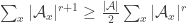There’s a neat way to rewrite this as follows by interchanging sums: $\sum_x |\mathcal{A}_x|^r = \sum_x \sum_{A_1,\ldots,A_r\in\mathcal{A}} \delta(x\in\bigcap_i A_i) = \sum_{A_1,\ldots,A_r} |A_1\cap\ldots\cap A_r|$ . Therefore the inequality above simply states that the average size of the intersection of $r+1$ uniformly chosen sets in $\mathcal{A}$ is at least half of the average size of the intersection of $r$ uniformly chosen sets in $\mathcal{A}$ .

For $r=0$ , this states that the uniformly averaged abundance is at least 1/2, which we know to be false. For $r=1$ , the inequality is $2\mathbb{E}_{A,B} |A\cap B|\geq \mathbb{E}_A|A|$ . This is a strengthening of FUNC that does not have any known counterexamples. (At least according to the paper, and I’ve also just checked this by computer on some of our running examples.) Moreover, there are several nice ways of rewriting it further, such as this one: $3\sum_{A,B} |A\cap B|\geq \sum_{A,B} |A\cup B|$ .

I figured that I’d mention this strengthening in case that somebody here hasn’t seen the paper but might know how to look for a counterexample. Since I personally find the lattice formulation to be the one which formalizes the relevant structures most accurately, I’ll keep thinking along these lines.
- Uwe Stroinski Says:
  March 7, 2016 at 2:11 pm
  The Duffus Sands example (p. 22 survey)
- Uwe Stroinski Says:
  March 7, 2016 at 2:43 pm
  Oops. The last comment was not meant to be sent before my computations have finished. They are still running. I expect $r = 1$ to be hit for $t=4$ .
- Uwe Stroinski Says:
  March 7, 2016 at 2:57 pm
  For $t =4$ we have 272 elements in $\mathcal{A}$ on a 24 element ground set. For $r = 1$ I get $\sum |A_x|^2 = 167384 < 175168 = 136 \sum |A_x|$ .
- Eckhard Says:
  March 9, 2016 at 4:39 pm
  I suppose that same example would also defeat the conjecture for fixed $r>1$ ? It might become computationally infeasible very quickly, but maybe a general proof is possible.
- Tobias Fritz Says:
  March 29, 2016 at 2:24 pm
  I’m interested in seeing examples of families in which the ratio $\frac{\mathbb{E}|A\cap B|}{\mathbb|A|}$ becomes arbitrarily small. Any ideas?
  
  Let me briefly explain why I think that the Duffus-Sands example doesn’t provide this. Recall that it consists of a power set of size $2^{2t}$ plus a totally ordered tail of size $2^t$ . This tail is exponentially small relative to the power set. We therefore should have $\mathbb{E}|A| = t + \tfrac{1}{2} + o(1)$ , since a random family member belongs to the power set most of the time and then contributes an average size of $t$ , while with a probability of about $2^{-t}$ it belongs to the tail and then contribute an average size of $2^{t - 1}$ plus lower-order terms. On the other hand, we will get $\mathbb{E}|A\cap B| = \tfrac{t}{2} + o(1)$ , corresponding to only the contribution of the power set: the exponential tail can make a significant contribution only if both $A$ and $B$ are in there, but this has a probability of roughly $4^{-t}$ , which is too small to be relevant. In conclusion, I would expect 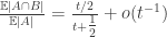$\frac{\mathbb{E}|A \cap B|}{\mathbb{E}|A|} = \frac{t/2}{t+\tfrac{1}{2}} + o(t^{-1})$ , which converges to 1/2 as $t\to\infty$ .
- Tobias Fritz Says:
  March 29, 2016 at 3:12 pm
  Sorry, that should have been $\frac{\mathbb{E}|A\cap B|}{\mathbb{E}|A|}$ in the first paragraph.
  
  And I forgot to mention that I’m only interested in families that separate points. (I usually think in terms of lattices, where this is automatic.)
Tobias Fritz Says:
March 5, 2016 at 10:23 pm | Reply
As it turns out, the MathOverflow question linked to in the main post comes surprisingly close to a proof of FUNC conditional on the finite lattice representation problem.

Proposition: Assuming a positive answer to the finite lattice representation problem, FUNC holds if and only if the following is true: for every finite group $G$ and subgroup $H$ , there is another subgroup $K$ that contains $H$ which is included in at most half of the subgroups that contain $H$ .

Proof sketch: By a result of Pálfy and Pudlák (see link above), a positive answer to the finite lattice representation problem implies that every finite lattice is isomorphic to the lattice of subgroups of some finite group $G$ that are above some subgroup $H$ . Hence what looks like a special case of FUNC is actually general. QED.

So, concerning further strategy I would like to propose this: we try to find a conditional proof of FUNC by looking at subgroup lattices of finite groups in more detail. Building on what has been done on MO, this seems reasonably concrete to do and it should be fun to learn some more group theory along the way. I’m hoping that it’s still easy enough to be doable. But I might be overly optimistic as usual 😉
- Tobias Fritz Says:
  March 5, 2016 at 10:30 pm
  Now that I’m reading the MathOverflow discussion in detail, I’m noticing that my proposal is basically what the OP there was saying. Sorry about being too overzealous with posting here… I’ll try to do my homework from now on.
- Tobias Fritz Says:
  June 14, 2016 at 3:18 pm
  In the meantime, the participants of the MathOverflow discussion have written a joint paper establishing FUNC for subgroup lattices of finite groups. Let me try to summarize their argument here.
  
  The proof is based on establishing FUNC for a class of lattices which includes many other classes for which FUNC has been proven as special cases. An element $m\in\mathcal{A}$ is left-modular if $a\leq b$ in $\mathcal{A}$ implies $a\lor (m\land b) = (a\lor m)\land b$ . There’s a short and sweet argument showing that if $\mathcal{A}$ has elements $m,x,y$ such that $m\neq 1$ is left-modular and $m\lor x\lor y =1$ , then $x$ or $y$ has abundance at most 1/2, so that FUNC holds. (The authors forgot to state the assumption $m\neq 1$ , but told me that this will be fixed in an upcoming revision.)
  
  The main group-theoretical ingredient is very simple to state, but very hard to prove: every nonabelian finite simple group is generated by an element of order 2 and an element of prime order. There seems to be a long history in group theory of establishing special cases of this result, while the last few cases have been finished off only very recently by King. This result implies, via a bit of elementary group theory, that subgroup lattices fall into the class of lattices described above.
Panurge Says:
March 7, 2016 at 9:59 am | Reply
In a comment about FUNC4, Thomas Bloom noted that if $F$ is a union-closed family with $m$ members, then Frankl’s conjecture “trivially implies that, for every $k\leq \log_2 m$, there exists some $k$-set which has abundancy at least $1/2^k$.” (In other words, there is a $k$-set contained in at least $m/2^k$ members of $F$.)
He added: “Note that the other extremal case, when $k=\log_2m$, is trivially true.”
If $k$ is not equal to $\log_2m$, the “other extremal case” seems less trivial to me. I posted an inelegant proof (without use of Frankl’s conjecture, of course) on Mathoverflow :

http://mathoverflow.net/questions/232757/literature-about-a-property-of-union-closed-families/232988#232988

and Fedor Petrov posted an elegant one. I also indicated a statement that seems likely to me and that would implie let us say the first half of the second extremal case in Thomas Bloom’s induction. I don’t know if this can interest specialists.
Alec Edgington Says:
March 7, 2016 at 11:38 am | Reply
A slight recasting of the Horn-clause representation gives us a duality between families over a ground set $X$ , on the one hand, and functions $2^X \to 2^X$ , on the other. This duality also gives a context to the ‘subgroups’ case of FUNC. Maybe it could lead to an alternative formulation of the conjecture.

I’ll focus on intersection-closed families here, since it seems easier to understand in those terms.

If $f$ is any function $2^X \to 2^X$ , let $\alpha(f)$ be the family of subsets $A \subseteq X$ such that for all $S \subseteq A$ , $f(S) \subseteq A$ . In the other direction, if $\mathcal{A}$ is a family of sets, let $\beta(\mathcal{A})$ be the function taking a set $S$ to the intersection of all $A \in \mathcal{A}$ such that $S \subseteq A$ .

Call a function $f : 2^X \to 2^X$ ‘beta-closed’ if:

$S \subseteq f(S)$ for all $S$ ; and
$f(T) \subseteq f(S)$ for all $T \subseteq f(S)$ .

For two functions $f, g : 2^X \to 2^X$ , say $f \leq g$ if $f(S) \subseteq g(S)$ for all $S$ .

Let the ‘beta-closure’ of $f$ be the minimal beta-closed function $g \geq f$ .

(I’m making up terminology as I don’t know if there’s an existing term for such functions.)

I think we then have the following facts:

$f \leq g \Rightarrow \alpha(f) \supseteq \alpha(g)$ and $\mathcal{A} \subseteq \mathcal{B} \Rightarrow \beta(\mathcal{A}) \geq \beta(\mathcal{B})$ ;
$\alpha(f)$ is intersection-closed for any function $f$ ;
$\beta(\mathcal{A})$ is beta-closed for any family $\mathcal{A}$ ;
$\alpha(\beta(\mathcal{A}))$ is the intersection-closure of $\mathcal{A}$ ;
$\beta(\alpha(f))$ is the beta-closure of $f$ ;

Is there a good way to translate FUNC to a statement about beta-closed functions?

Note that we can easily express the ‘subgroups’ case of FUNC in this setting: if $X$ is a group, let $f(S)$ be the subgroup generated by $S$ . Then $\alpha(f)$ is the family of all subgroups of $X$ .
- Tobias Fritz Says:
  March 8, 2016 at 11:09 pm
  Maybe it’s worth saying that such functions are usually called closure operators, and it is well-known that these correspond to intersection-closed families; see the section “Closed sets” in the Wikipedia article. The properties that you mention are arguably due to $\alpha$ and $\beta$ forming a Galois connection between set families and functions, in the sense that $\mathcal{A}\subseteq\alpha(f)$ if and only if $f\leq\beta(\mathcal{A})$ . (To see this, note that both of these statements simply say that $S\subseteq A$ must imply $f(S)\subseteq A$ for $A\in\mathcal{A}$ .)
  
  I haven’t found a good way to translate FUNC to a statement about closure operators, where I interpret “good” as meaning that it doesn’t just replace one term for another, but also provides a fresh perspective.
  
  Oh, could you expand a bit on what relation you see between this and the Horn clause picture?
- Alec Edgington Says:
  March 9, 2016 at 8:56 am
  Ah, thanks.
  
  To explain the connection with Horn clauses, I’ll use the shorthand notation from FUNC3, writing $(x,S)$ as shorthand for the condition $x \in A \Rightarrow A \cap S \neq \emptyset$ . Translating the above from the intersection-closed to the union-closed setting, the mapping from a family $\mathcal{A}$ to a closure operator $f = \beta^\prime(\mathcal{A})$ becomes $f(S) = \{x : (\forall A \in \mathcal{A}_x) A \cap S \neq \emptyset\}$ . In other words, $f(S)$ is the set of $x$ such that $(x,S)$ .
gowers Says:
March 8, 2016 at 12:11 pm | Reply
I haven’t quite worked out how this relates to some of the discussion above about moments, but here is a simple observation that suggests that insisting that set systems separate points doesn’t really make a fundamental difference to what kinds of arguments work and what don’t. (I won’t try to make that claim precise.) I have a feeling I may have said this already, in which case apologies for the accidental repetition.

Let $m$ and $n$ be positive integers with $n$ much less than $m$ and $m$ much less than $2^n$ . Build a union-closed family $\mathcal A$ on $[m]$ as follows: it consists of all subsets of $[n]$ together with all subsets of $[m]$ of cardinality at least $m-1$ .

This set system contains $2^n+m+1$ sets. If $x\in [n]$ then it belongs to $2^{n-1}+m$ sets, while if $x\notin [n]$ then it belongs to $m$ sets. Since $m$ is much less than $2^n$ , the abundance of each $x\in [n]$ is roughly 1/2 and the abundance of each $x\notin [n]$ is roughly 0. Therefore, since $n$ is much less than $m$ , the average abundance is roughly 0, and this will be true of higher moments as well.

In other words, the same sort of example that kills off naive averaging arguments kills off the same naive averaging arguments even if one insists on a set system that separates points.
Tobias Fritz Says:
March 9, 2016 at 10:39 am | Reply
It turns out that the Horn clause formulation for intersection-closed families is actually well-known in the literature on formal concept analysis and related areas; I’ve learnt about this from reading this paper, where it is essentially shown that Tim’s canonical system of Horn clauses based on the minimal transversals of $\mathcal{A}_x$ coincides with several other definitions of canonical systems that had been proposed previously. The authors quote a 1992 paper of Dechter and Pearl, who state that the equivalence between Horn functions and families of subsets closed by intersection “appears to be a general folklore among many researchers, although we could not trace its precise origin”.

Since it’s been getting a bit more difficult to keep track of the entire discussion so far, I’ve been expanding the wiki a bit and am currently working on a page describing the Horn clause formulation. [Not posting the link in order not to trigger the spam filter. You can get there from the Polymath11 main page.]
Tobias Fritz Says:
March 18, 2016 at 10:06 am | Reply
Here’s a quick summary of what I’ve been thinking about in terms of the lattice formulation. A decent part of this is on the wiki. If anyone wants to see more details on anything and/or join the fun, I’d be happy to elaborate and discuss things.

1) It is sufficient to consider atomistic lattices only. In terms of the standard formulation in terms of union-closed families, this means that we can always assume that all sets of the form $X\setminus\{x\}$ belong to $\mathcal{A}$ . This answers a question that had come up at FUNC3.

2) While I still don’t know whether weighted FUNC follows from FUNC, there now is a proof that weighted FUNC with every weight a power of 2 follows from Poonen’s strong FUNC, i.e. the assertion that every union-closed family has an element of abundance strictly larger than 1/2 or is (isomorphic to) a power set.

3) Here’s another strengthening that may be of interest:

Poset FUNC: let $\mathcal{P}$ be an arbitrary finite poset with $|\mathcal{P}|\geq 2$. Then $\mathcal{P}$ contains a join-irreducible element of relative abundance $\leq 1/2$ .

While this survives the basic sanity checks, there may still be relatively simple or small counterexamples. Also, it seems likely that other people who have thought about the lattice formulation have considered this as well, although I don’t think I’ve seen it mentioned anywhere.

4) I’ve been studying Wójcik’s proof of the best-known general abundance bound of $\frac{2.4 n}{\log_2 n}$ , and from my perspective it is lattice-theoretic in nature. In fact, part of what Wójcik does is to identify a large subsemilattice in $\mathcal{A}$ that decomposes naturally as a fibre bundle. The challenge here is to make this subsemilattice as large as possible relative to $\mathcal{A}$ . So while I had proposed at FUNC3 to look for fibre bundle decompositions of $\mathcal{A}$ itself and had to realize that these do not always exist, Wójcik has (possibly unknowingly) implemented a refinement of this idea that gives something interesting.
- Uwe Stroinski Says:
  March 18, 2016 at 4:06 pm
  I am interested in details (especially on 1) and 4)).
- Tobias Fritz Says:
  March 18, 2016 at 6:31 pm
  Great! So here’s some more info on 1); I’ll write more about 4) tomorrow.
  
  The proof of 1) in the lattice formulation is at the wiki page
  that I had linked to above; but the proof translates easily into the
  conventional picture and it is quite simple, so let me present it here.
  I’m considering $c$ -FUNC for a constant $c\leq 1/2$ as the
  assertion that there always exists an element of abundance at least
  $c$ ; if you like, you can specialize to the case $c=1/2$ and
  only consider standard FUNC.
  
  Lemma: If there $\varepsilon > 0$ such that $c$ -FUNC
  holds when $|X|\leq \varepsilon |\mathcal{A}|$ , then it holds in general.
  
  Proof: To derive $c$ -FUNC for an arbitrary $\mathcal{A}\subseteq 2^X$ , consider the $k$ -fold product $\mathcal{A}^k$ as in the main post of FUNC2. This lives on a ground set
  which consists of $k$ disjoint copies of $X$ , and the
  different abundances of the elements are the same as those of the
  original $\mathcal{A}$ . Now notice that $|\mathcal{A}^k|$
  grows exponentially while the size of the ground set grows only linearly
  in $k$ , so that we can make the quotient of these cardinalities
  arbitrarily small.
  
  Proposition: If $c$ -FUNC holds for every $\mathcal{A}\subseteq 2^X$ which contains all sets $X\setminus\{x\}$ , then it holds in general.
  
  Proof: Simply throwing in those sets creates a union-closed family $\mathcal{A}'$ , for which we assume a lower bound on maximal abundance of $|\mathcal{A}'_x|\geq c|\mathcal{A}'|$ . Also, we can assume $|X|\leq \varepsilon |\mathcal{A}|$ by the lemma. Therefore $\frac{|\mathcal{A}_x|}{|\mathcal{A}|} \geq \frac{|\mathcal{A}'_x| - |X|}{|\mathcal{A}'|} \geq \frac{c|\mathcal{A}'| - \varepsilon|\mathcal{A}|}{|\mathcal{A}'|} \geq c-\varepsilon$ . Since $\varepsilon$ was arbitrary, the claim follows.
- Tobias Fritz Says:
  March 19, 2016 at 7:22 am
  I’d appreciate it if somebody could go through the above argument to make sure that it’s ok. Sorry about the messy formatting, that wasn’t intended…
  
  I forgot to mention that Poset FUNC should also assume $\mathcal{P}$ to have a least element. Otherwise, taking a power set and removing the empty set results in a counterexample.
- Tobias Fritz Says:
  March 19, 2016 at 12:38 pm
  The wiki now contains some details on 4). We can discuss anything that may be unclear.
  
  Besides obtaining a better structural understanding of finite lattices, my goal in extracting these general statements from Wójcik’s proof is to try and improve on his bound of $\frac{2.4\log_2 n}{n}$ . Of course this is unlikely to be possible with his very techniques, since otherwise he would already have done so, but it’s still good to have these tools at hand and maybe we’ll figure out how to sharpen them.
- Uwe Stroinski Says:
  March 21, 2016 at 12:30 pm
  1) is very nice. Ad 4) I have to do some homework concerning lattices. I willing to do that, since this formulation of the problem seems to be optimal to make it accessible to automated reasoning. This view of mine might be very, very naive, but one reason why at least I cannot post a lot on this problem is that whatever I do I get a lot of “boring” cases without many ideas. For others that might be similar. Why not turn this property against the problem?
  
  In any case, I share your opinion on Woicik’s proof.
- Tobias Fritz Says:
  March 21, 2016 at 3:02 pm
  Sounds good! I share your general feeling about the problem: it’s very hard to come up with good ideas that don’t pretty soon run into a wall…
- Sean Says:
  June 8, 2017 at 3:02 pm
  Apologies in advance if the project is no longer active, or if I have missed something obvious.
  
  I think I’m missing something in my understanding of the proof of (1). I thought I followed the argument, but then saw no obstacle to extending it to a further result which seems too good to be true. Call a union-closed family “r-complete” if it contains all of the sets of size (n-r). Then the result on atomistic lattices being sufficient to consider is equivalent to saying it is enough to consider 1-complete families (no doubt there is a lattice-theoretic term for this).
  
  We want to show that if c-FUNC works for all r-complete families, it holds for all (r-1)-complete families.
  
  Take an arbitrary (r-1)-complete family, $\mathcal{A}$ , $n=\left| X \right|$ . At most $\left(\begin{array}{c}n\\ r\end{array}\right)$ sets need to be added to turn $\mathcal{A}$ into an r-complete family $\mathcal{A'}$ , still union-closed since $\mathcal{A}$ was (r-1)-complete. We want to follow the same series of inequalities as much as is possible in the original proof, so want $\left(\begin{array}{c}n\\ r\end{array}\right) < \epsilon \mathcal{A}$ . If we don’t have this for $\mathcal{A}$ , then replace with $\mathcal{A}^k$ for a sufficiently large power k as in the lemma; $\left(\begin{array}{c}kn\\ r\end{array}\right)$ is eventually small compared to $\mathcal{A}^k$ which is at least $\left(\begin{array}{c}n\\ r-1 \end{array}\right)^k$ as $\mathcal{A}$ is (r-1)-complete. Such an $\mathcal{A}^k$ is still union-closed and (r-1)-complete with abundances preserved. So we go ahead and form $\mathcal{A}'$ ; by our initial assumption we may choose $x$ with $\left|\mathcal{A}'_x \right| > c\left|\mathcal{A}'\right|$ .
  
  The argument then continues largely as before:
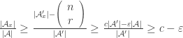  $\frac{|\mathcal{A}_x|}{|\mathcal{A}|} \geq \frac{|\mathcal{A}'_x| - \left(\begin{array}{c}n\\ r\end{array}\right)}{|\mathcal{A}'|} \geq \frac{c|\mathcal{A}'| - \varepsilon|\mathcal{A}|}{|\mathcal{A}'|} \geq c-\varepsilon$ . QED
  
  This sounds to good to be true. As I said, I have probably overlooked something obvious.
gowers Says:
March 18, 2016 at 10:51 am | Reply
The rate of comments has slowed down a lot recently: Tobias’s comment is the first for a few days. So I think we should decide what to do now. Here are the options as I see them.

1. We decide that the project has run out of steam, devote some effort to writing a nice document about the various different ideas that have been discussed, post it to the arXiv, and declare the project closed.

2. We do the above, up to but not including the last two steps, and then see whether the writing of the document stimulates us to continue the discussion further (as it easily might, as writing a document tends to draw attention to lots of loose ends).

3. We declare that Polymath11 is closed, but start a new and more private project to continue working on FUNC, with anybody who wishes to participate and can promise at least some commitment to participating (at a level similar to the level of commitment that one would have to a conventional mathematical collaboration).

4. We just continue as at present and hope that the rate of comments picks up.

The fourth option isn’t necessarily hopeless: part of the reason I have not commented much recently is that I have been busy with a number of other things, and it may be that I could get the conversation going again if I set aside some time to write a new post and make regular contributions to the ensuing discussion.

Anyhow, thoughts, particularly from people who have made a lot of comments on Polymath11, would be very welcome.

The only thing I want to avoid is drifting without making a clear decision about what our policy is. That has happened in the past, and I think it is better to finish projects in a clean way if they are going to finish.
- Markus Sigg Says:
  March 18, 2016 at 11:01 am
  I think it does not hurt to keep this open for a few more weeks or months.
- Tobias Fritz Says:
  March 18, 2016 at 4:43 pm
  I wholeheartedly agree with Tim’s last sentence on finishing projects in a clean way. I’m personally open to either of those four options, and also to Markus’s suggestion of leaving this open for a bit longer. I’m pretty sure that if we attempt 1., then I couldn’t help myself thinking further about the problem. But of course I could restrain myself to doing so in private if you guys prefer to finish things up.
  
  Currently my gut feeling is that of having obtained a decent amount of understanding of the problem comparable to what’s in recent literature. There are many further avenues to explore, which I’m eager to do, and this may result in something new. But I don’t have any lead that would hold the promise of a major breakthrough.
Uwe Stroinski Says:
March 18, 2016 at 4:26 pm | Reply
Closing a polymath project before it is really dead might have a negative impact on future projects.
gowers Says:
March 18, 2016 at 8:52 pm | Reply
Based on the above comments, I think the best thing is not to do anything for now. I won’t be able to contribute much between now and about April 10th, but at that point I will try to catch up with the current lines of thought (as they are then), write a new post, and make regular contributions for a while after that. There are still questions that I feel I could think about a lot harder than I have so far, so I think I will be able to come up with things to say.

The main reason for not wanting a project to drift on for too long in an inactive state is that it leaves people who want to work on the problem in future in an awkward position. But if at some point we mark the end of a project by writing a preprint, which might even be publishable, then people have something to refer to and there is no awkwardness about assigning credit to any ideas that might have arisen in the project.
- Gil Kalai Says:
  March 19, 2016 at 7:12 pm
  Let me mention the situation regarding polymath 10 which is running on my blog. (In a slower paste compared to polymath11.) I hope to come back to it soon, and, of course, further comments on post 4 are most welcome. (I hope to be able to report on some computer experimentation regarding the various conjectures and ideas.) In April I am planning to launch a fifth post.
  
  Overall I consider one year as a good time span for that project, but I agree that a clear end-of-project deceleration and some effort to organize the results could be useful. We can even decide that as a default a polymath project terminates one year after it starts.
  
  Of course, I regard it perfectly ok/welcome if people work on the problem in parallel to the polymath, and even if they pursue some avenues discussed there on their own.
- gowers Says:
  March 19, 2016 at 9:54 pm
  Thank you for sharing that. I think that for FUNC a year may be a bit too long, unless things pick up again. But I now think that the best option for FUNC is probably option 2: that is, write up the discussion so far but in the hope that it stimulates further progress. And then if it doesn’t, it will be easy to close the project and say that the document is its write-up.
Tobias Fritz Says:
March 20, 2016 at 8:03 am | Reply
I can now formulate the problem of fnding a fibre bundle inside some union-closed family $\mathcal{A}\subseteq 2^X$ also in conventional language (without lattices). The idea of finding a bundle inside is to exploit this structure in order to derive lower bounds on maximal abundances. This is part of what Wójcik did in deriving the best-known unconditional bound of $\frac{2.4n}{\log_2 n}$ . Obtaining good unconditional bounds seems to require identifying some kind of structure within $\mathcal{A}$ , and this is one way to do so. I wonder if one can use it to improve on Wójcik’s result.

For now, let me just present a special case of the question which recovers e.g. the fibre bundle decomposition of Thomas Bloom‘s example. Namely, how does one need to choose $B\in\mathcal{A}$ such that $A\setminus B\in\mathcal{A}$ for as many $A\in\mathcal{A}$ as possible? And for an optimal choice of $B$ , what is the number of $A$ ‘s for which this holds?

In Thomas’s example, choosing $B=\{1,2,3,4,5,6\}$ means that $A\setminus B\in\mathcal{A}$ for every $A\in\mathcal{A}$ , so that the entire $\mathcal{A}$ decomposes as a fibre bundle.

[PS: if anyone feels that I’m cluttering the discussion too much, please let me know! Then I’ll comment less and put things on the wiki instead.]
Tobias Fritz Says:
March 21, 2016 at 3:07 pm | Reply
To try and restart the discussion, let me present an idea that doesn’t rely on lattice theory, but rather has a dynamical systems and automata theory flavour. Let $\mathcal{A}\subseteq 2^X$ be a union-closed family, and let’s try to prove FUNC by induction on $|X|$ . So we need to show that there exists some $x\in X$ with $|\mathcal{A}_x|\geq|\mathcal{A}_{\bar{x}}|$ .

The base case $|X|=1$ is trivial, so let’s focus on the induction step. By the induction assumption, for every $x$ we have some $f(x)$ such that 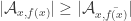$|\mathcal{A}_{x,f(x)}|\geq |\mathcal{A}_{x,\bar{f(x)}}|$ . Similarly, we have $g(x)$ such that $|\mathcal{A}_{\bar{x},g(x)}|\geq |\mathcal{A}_{\bar{x},\bar{g(x)}}|$ . We can now consider these two maps $f,g:X\to X$ as a finite automaton on the input alphabet $\{f,g\}$ . One can easily complete the induction step in at least the following cases:

1) There is $x$ such that $f(x) = g(x)$ . Then we have $|\mathcal{A}_{f(x)}| = |\mathcal{A}_{x,f(x)}| + |\mathcal{A}_{\bar{x},f(x)}| \geq |\mathcal{A}_{x,\bar{f(x)}}| + |\mathcal{A}_{\bar{x},\bar{f(x)}}| = |\mathcal{A}_{\bar{f(x)}}|$ , and we are done.

2) There is $x$ such that $g(f(x)) = x$ . Putting $y:=f(x)$ then results in $x = g(y)$ , so that we have $|\mathcal{A}_{xy}|\geq|\mathcal{A}_{x\bar{y}}|\geq|\mathcal{A}_{\bar{x}\bar{y}}|$ .

Now the questions are: What’s an example of a small automaton for which neither of these conditions holds? (Note that we also must have $f(x)\neq x\neq g(x)$ for all $x$ .) Are there other cases in which the induction step can be completed easily?

Of course, to complete the induction step in general one will most likely have to use union-closure in a stronger sense. In what way could this possibly come in? Can we combine this idea with Tom Eccles’ approach?
- Tobias Fritz Says:
  March 21, 2016 at 3:10 pm
  I forgot to say that the induction step in case 2) uses Miroslav’s argument to conclude FUNC from $|\mathcal{A}_{xy}|\geq|\mathcal{A}_{\bar{x}\bar{y}}|$ .
- Miroslav Chlebik Says:
  March 21, 2016 at 5:02 pm
  I would like to mention that the “local averaging argument”, that I used earlier for the pairs, in more general context can be also useful. Namely, given a union-closed family $\latex \mathcal A$ over the ground set X, we can try to prove the existence of an abundant element. We have seen earlier the situations when it is “easier” to identify first a larger set $\latex A \subset X$ for which we are able to prove existence of an abundant vertex in it. If we define an “excess” of a set
  $\latex A \subset X$ by
  $\latex e(A)=\sum_{x \in A} |\mathxal A_x|-|\mathcal A_{\bar x}|$, then FUNC for $\latex \mathcal A$ is equivalent to the existence of a nonempty set $\latex A \subset X$ with $\latex e(A) \geq 0$ (with $\latex e(A) > -|A|$ would be also enough).
  While this is clearly equivalent question, I demonstrated that sometimes it may be “more natural” to prove this for larger set A (a pair, for example) and not for a singleton.
- Tobias Fritz Says:
  March 22, 2016 at 9:22 am
  If I understand correctly, this kind of local averaging has also been used by Poonen in his study of set configurations that imply FUNC (in particular p.5/6), so it seems like a useful tool to have at hand.
  
  Let me describe what I was trying to do yesterday a bit differently. Construct a directed graph on the vertex set $X$ with edge labels ‘blue’ and ‘red’ as follows. If $|\mathcal{A}_{xy}|\geq |\mathcal{A}_{x\bar{y}}|$ , then put a blue edge $x\to y$ , which stands for $y$ being abundant in $\mathcal{A}_x$ . If $|\mathcal{A}_{\bar{x}y}|\geq |\mathcal{A}_{\bar{x}\bar{y}}|$ , then put a red edge $x\to y$ , which stands for $y$ being abundant in $\mathcal{A}_{\bar{x}}$ . The induction assumption guarantees that every vertex has at least one outgoing edge of each colour. It may help to think of this directed graph as the set of transition rules of a finite automaton (nondeterministic and with binary input).
  
  My idea was to find subgraph configurations that would guarantee FUNC, such as a blue edge parallel to a red edge (case 1) or a blue edge antiparallel to a blue edge (case 2). But so far I haven’t been able to find any configuration of at least three vertices and without (anti-)parallel edges from which FUNC would follow. So it may well be that the whole idea is totally naive and kind of trivial; I’m not sure.
- Miroslav Chlebik Says:
  March 22, 2016 at 12:50 pm
  I have used the term “local averaging” to stress that we may need to consider averaging over any subset A of a ground set X (rather than over the whole ground set X.)
  Given a union closed family $\mathcal A$ over a ground set X, and keeping a set $A \subset X$ fixed, we can partition sets in $\mathcal A$ according to their traces in A. For any $D \subset A$ we consider sets
  $B \in \mathcal A$ with $B \cap A=D$ . To be consistent with previously used notation this subfamily can be denoted $\mathcal A_{D, \bar {A \setminus D}}$ .
  Now it is easy to express $\sum_{x \in A} |\mathcal A_x|$ , $\sum_{x \in A} |\mathcal A_{\bar {x}}|$ and $e(A)$ using this partition; for example,
  $ $e(A)=\sum_{D: D \subset A} (2|D|-|A|) |\mathcal A_{D\bar{A \setminus D}}.$ $
  An example, when $A=\{x, y\}$ , was what I used earlier,
  and then $ $e(A)=2(|\mathcal A_{xy}|-|\mathcal A_{\bar{x}\bar{y}}|)$ $.
  Indeed, sometimes it is easier to prove that $e(A) \geq 0$ on the way to prove that (at least) one of x, y is abundant; this is how this local averaging can help even in higher generality.
- Tobias Fritz Says:
  March 22, 2016 at 1:18 pm
  Is that just a further elaboration or specifically a reply to my comment?
  
  (Maybe you had the impression that I had misunderstood something. If this is the case, then I might have expressed myself badly. Was anything unclear about what I said and I should elaborate? These things are hard to gauge online, which is why I’m asking explicitly.)
Miroslav Chlebik Says:
March 22, 2016 at 1:35 pm | Reply
I haven’t started to comment on you last attempt (I am sorry for that), but I wanted (and still will continue) to put few more (related) ideas that haven’t been considered enough (in my opinion), to prevent this project closure prematurely if we see new avenues of research that deserve our attention.
- Tobias Fritz Says:
  March 22, 2016 at 1:52 pm
  No need to be sorry, I just wanted to make sure that we’re not miscommunicating. Looking forward to see what you have in mind!
- Uwe Stroinski Says:
  March 23, 2016 at 10:16 am
  Concerning local averaging. Tobias’s inequality implies FUNC for the extreme cases, i.e. the existence of either small or large minmal all-intersecting sets.
  
  The known counterexamples to averaging have either a small all-intersecting set (Duffus-Sands) or a large all-intersecting set (Hungarian familiy). Thus, in the region where we know that averaging does not yield FUNC we get FUNC from the inequality.
  
  I have not yet thought very much about it, but the following question seems to be natural: Can we get an averaging argument over medium sized minimal all-intersecting sets to work?
- Tobias Fritz Says:
  March 23, 2016 at 4:15 pm
  That’s an interesting observation. The general idea of distinguishing various regimes seems to be a good one: for example, it was applied successfully to FUNC in this impressive paper.
  
  On the other hand, my inequality can at most establish weak FUNC, since it leads to an abundance bound of 1/2 only in the trivial cases where some minimal all-intersecting set has size at most 2 or exactly $\log_2|\mathcal{A}|$ . But we can still try to use your idea to attack weak FUNC. For doing this, I suspect that an averaging argument can also establish weak FUNC when there is a large minimal all-intersecting set: the Hungarian family has average abundance close to 1/2, and in general a family in which all minimal all-intersecting set are large should be close to a power set in some sense. So if your hypothesis is correct, then the regime in which averaging does not always establish weak FUNC is probably when there is a small all-intersecting set. And in this case, my inequality is only a negligible improvement over Knill’s original bound, so we might as well use the latter (simpler) one.
  
  In summary, it seems interesting to distinguish two regimes:
  
  1) There is a small all-intersecting set (minimal transversal), say of cardinality $|S|\leq \frac{\log_2 n}{3}$ . Then Knill’s bound establishes a maximal abundance of at least $\frac{3(n-1)}{\log_2 n}$.
  
  2) Suppose that every all-intersecting set has cardinality $|S| > \frac{\log_2 n}{3}$ . Does this imply an average abundance of at least $\frac{3n}{\log_2 n}$ ?
  
  A positive answer to 2) would yield a slight improvement over Wójcik’s best-known bound to $\frac{3n}{\log_2 n}$ . Of course I’ve chosen the numbers precisely such that this comes out, and the exact numbers should be adapted to whatever we can achieve. Moreover, by my earlier observations we can assume wlog that $\mathcal{A}$ contains all sets $X\setminus\{x\}$ , which also removes the ambiguity of duplicating elements and forces $\mathcal{A}$ to be separating.
- Tobias Fritz Says:
  March 23, 2016 at 6:08 pm
  Actually it’s not even true that the Duffus-Sands example has a small all-intersecting set: the unique minimal all-intersecting set is $V$ , with cardinality $|V| = 2t$ . This is definitely not small relative to $\log_2|\mathcal{A}| = latex \log_2(2^{2t} + 2^t)\approx 2t$ . Hence Knill’s argument does not lead to any good bound on the maximal abundance, but my inequality surprisingly does give the desired $|\mathcal{A}|/2$ as $t\to\infty$ . All this has to do with the fact that the Duffus-Sands example is very close to a power set: you only need to remove an exponentially small number of members to arrive at the power set $2^V$ .
  
  I’m not sure yet what this implies for averaging. One encouraging (but probably unrelated) fact is that the paper that I linked to above relies on averaging throughout.
Uwe Stroinski Says:
March 24, 2016 at 7:17 am | Reply
You are of course right with Duffus-Sands having a large minimal all intersecting set and yes weak FUNC should be the target.

I still think that averaging might work in the correct regime and will try to post some maths showing that later today.
- Uwe Stroinski Says:
  March 24, 2016 at 7:17 am
  My last comment was meant as a replay to Tobias.
Miroslav Chlebik Says:
March 24, 2016 at 11:36 am | Reply
I tend to think about a potential induction proof in a way that I would like to understand many properties of a “minimal counterexample” (we can think of more natural partial orders,
the size $n=\mathcal A$ is just one of options), and then we want to show, to get a contradiction, that given such a minimal counterexample we are always able to find a smaller one.
So consider our “minimal counterexample” $\mathcal A$ with a ground set X, consider a minimal hitting set (transversal)
$S \subset X$ . We certainly can find a subfamily $\mathcal B$ of $\mathcal A$ whose traces in S reproduces the power set $2^S$ . If the estimate $|S| \leq log_2(n)$ would be our only use of the fact that we deal with “union-closed families”, then we can hardly improve the Knill’s result. But the fact that the traces of $\mathcal B$ in S form the power set $2^S$ suggests that “removing” $\mathcal B$ from $\mathcal A$ should result in a smaller counterexample; the contradiction. Of course, this is not so simple, as we could get into the families that are not “union-closed”. Alternatively, one can think about weighted (and even weaker) versions of FUNC in this “minimal contradiction” scenario; then try to get weight 0 to sets in $\mathcal B$ (but be carefull what other weights need to be modified then as well), and look if we can find still a smaller counterexample this way.
Uwe Stroinski Says:
March 24, 2016 at 6:38 pm | Reply
To outline the above mentioned idea let me first sketch a lattice–free proof of Tobias’s inequality to keep this coment somewhat self–contained.

Let $S$ be a minimal subset of $U(\mathcal{A})$ such that any non–empty set $A\in\mathcal{A}$ has non–empty intersection with $S$ . Then

$\sum_{x\in S} |A_x|\geq |S| \frac{2^{|S|}}{2}+|\mathcal{A}|-2^{|S|}.$

Proof. Since $S$ is minimal there is for each $x\in S$ a set $A\in\mathcal{A}$ with $A\cap S=\{x\}$ . By union–closedness of $\mathcal{A}$ we obtain that $\{S\cap A:A\in\mathcal{A}\}$ is equal to the powerset of $S$ . Since the frequencies of all $|S|$ elements in the powerset are $\frac{2^{|S|}}{2}$ we get the first part. There are still $|\mathcal{A}|-2^{|S|}$ sets left and since they are non–empty and since $S$ has non–empty intersection with them we can bound the rest of the sum from below by $|\mathcal{A}|-2^{|S|}$ .

As already noted by Tobias, this bound implies

$\max_{x\in S}|A_x|\geq \left(\frac{1}{2}-\frac{1}{|S|}\right)2^{|S|}+\frac{|\mathcal{A}|}{|S|}.$

Let now $c$ –FUNC denote FUNC with 1/2 replaced by some $0<c\leq1/2$ .

Whenever there is a minimal all-intersecting set $S$ with $|S|\leq 1/c$ or $|S|\geq \log (2 c|\mathcal{A}|)$ , then $\mathcal{A}$ satisfies $c$ –FUNC.

Proof. The case $|S|=1$ is easy. For $1<|S|\leq 1/c$ we get that $\frac{1}{2}-\frac{1}{|S|}\geq 0$ and thus $\max_{x\in S}|A_x|\geq \frac{|\mathcal{A}|}{|S|}\geq c|\mathcal{A}|$ . For $|S|\geq \log (2 c|\mathcal{A}|)$ we get

$\left(\frac{1}{2}-\frac{1}{|S|}\right)2^{|S|}+\frac{|\mathcal{A}|}{|S|}\geq c|\mathcal{A}| +\frac{|\mathcal{A}|(1-2c)}{|S|}\geq c|\mathcal{A}|.$

Provided the above is correct we can apply it to e.g. Duffus–Sands. Here we have $|S|= 2t$ and $|\mathcal{A}|= 2^{2t}-2^t$ . Duffus–Sands then satisfies $\min_t \max\{\frac{1}{2t},\frac{1}{2(1+\frac{1}{2^t})} \}$ –Func. That is $\frac{2}{5}$ –FUNC, a result that cannot be achieved by averaging.

If we now could get a result in the spirit of Reimer (cf. Thm.21 survey) for the case that all minimal all–intersecting sets are smaller than $\log(2 c |\mathcal{A}|)$ , e.g. by a slick up–compression argument, we might make progress on $c$ –FUNC.

This is getting long and it is getting late. Let me conclude: modulo some technical hiccups I made, the idea is as follows. In the region where we know averaging to fail we prove $c$ –FUNC by Tobias's bound. In the other region we try to use averaging to prove $c$ –FUNC.
- Tobias Fritz Says:
  March 25, 2016 at 10:48 am
  After pondering this for a while, I think that this particular approach won’t work, for the following reasons:
  
  1) We already know that every minimal all-intersecting set has cardinality at most $\log_2(|\mathcal{A}|)$ (since all possible traces must occur). Hence assuming that every all-intersecting set has cardinality at most $\log_2(2c|\mathcal{A}|) = \log_2(|\mathcal{A}|) - |\log_2(2c)|$ gives us an assumption that’s better only by an additive constant.
  
  2) Here are some general observations on averaging that are easiest to explain in the lattice formulation. Naive averaging samples from the uniform distribution over all join-irreducibles. In this case, the average abundance is very sensitive to small modifications of the lattice that add or remove new join-irreducibles. More concretely, by gluing in a small number of new join-irreducibles at the bottom, one can make the average abundance increase arbitrarily. This is what happens in the Duffus-Sands example, where one glues a total order of size $2^t\ll |\mathcal{A}|$ to the bottom of a power set, and in Tim’s example who essentially glues a copy of the lattice $M_m$ also to the bottom of a power set. ( $M_m$ is the lattice that you get when you take a top and a bottom element and throw in $m$ mutually incomparable elements in between.)
  
  Of course, there are many other ways in which one could alter the average abundance while introducing only a small number of elements by adding new join-irreducibles. My conclusion is that there is no regime, specified only by some relation between the size of all-intersecting sets and $|\mathcal{A}|$ , in which averaging could work in all cases.
  
  This is why uniform averaging looks like too crude a tool. We might have more luck by doing a more clever sort of averaging. Certainly Miroslav’s local averaging can perform better, since it’s precisely what gives us Knill’s bound when applied to an all-intersecting set. However, it’s hard to find a suitable set $A\subseteq X$ with respect to which we should apply local averaging. How about choosing it at random as well, say uniformly chosen over all nonempty $A\in\mathcal{A}$ ? This is indeed not too bad, since it’s exactly Tim’s “average overlap density” proposal (see the main posts to FUNC1 and FUNC2).
  
  Now recall that Tim had found an example where the average overlap density was below 1/2. I believe that one can even apply his reasoning to Thomas Bloom’s family of examples to obtain arbitrarily small average overlap density. However, these counterexamples are heavily based on duplicating elements, and so far there is no counterexample that separates points (as far as I know). Moreover, assuming separation of points is actually a very natural condition from the lattice-theoretic perspective: duplicating elements does not affect the lattice structure of $\mathcal{A}$ , and in particular new duplicated elements of the ground set do not result in new join-irreducibles in the lattice. So if one formulates an average overlap density conjecture in terms of lattices, the problem of duplication of points will not even come up. But since most people are more comfortable with the set-based formulation, let me propose a revised average overlap density conjecture (implying weak FUNC) like this:
  
  Conjecture: There is $c>0$ such that if a union-closed family $\mathcal{A}\subseteq 2^X$ contains all sets of the form $X\setminus\{x\}$ , then $\mathcal{A}$ has an average overlap density of at least $c$ .
- Tobias Fritz Says:
  March 25, 2016 at 7:47 pm
  Here’s an argument which suggests that the conjecture is most likely false, together with a general lesson on averaging arguments. I’m going to gloss over some details, hoping that the principal thrust of the idea is correct.
  
  Suppose that the conjecture holds for a certain $c>0$ . Then let’s apply it to $\mathcal{A}^{\times N}$ , the $N$ -fold product of $\mathcal{A}$ with itself for some integer $N$ . In this new family, the average overlap density is the expectation value of
  $\frac{|A_1\cap B_1| + \ldots + |A_N\cap B_N|}{|A_1| + \ldots + |A_N|}$
  where these variables are iid copies of the original $A$ and $B$ . By the law of large numbers, this should converge to $\frac{\mathbb{E}_{A,B}|A\cap B|}{\mathbb{E}_A|A|}$ , although I haven’t worked this out rigorously. This is an expression that we’ve seen before. As Uwe’s computation revealed, this expression is less than 1/2 for the Duffus-Sands example with parameter $t = 4$ . Hence a suitably large power of the Duffus-Sands example should also show that my conjecture does not hold with $c = 1/2$ . Since it’s very likely that $\frac{\mathbb{E}|A\cap B|}{\mathbb{E}|A|}$ can get arbitrarily small, this probably refutes my conjecture completely.
  
  The general lesson is that a good averaging inequality should be well-behaved with respect to products, which the average overlap density inequality apparently is not. In contrast, the conjectural Duffus-Sands inequality, namely Eq. (2) in their paper “An inequality for the sizes of prime filters of finite distributive lattices”, is nicely stable under products.
Panurge Says:
March 29, 2016 at 6:13 pm | Reply
On this Mathoverflow page :

http://mathoverflow.net/questions/234759/frankls-conjecture-and-oeis-sequence-a188163

I suggested a link between Frankl’s conjecture and Oeis sequence A188163.
But i’s only a guess on a rather small basis.
- Tobias Fritz Says:
  March 29, 2016 at 6:41 pm
  This looks a lot like the discussion in Section 8 of the survey. If this is what you’re after, then it seems to be quite a good guess, but nevertheless one that becomes wrong eventually.
Panurge Says:
March 29, 2016 at 8:35 pm | Reply
Thanks for the answer, but I don’t understand it. What is Section 8 of the survey ? And do you mean that the relation f(c) = A188163(c) (in my notations) is false ? I’m sorry if I am importunate.
- Tobias Fritz Says:
  March 30, 2016 at 4:00 pm
  Judging by the comment thread over at MathOverflow, Panurge seems to have answered their own questions already, but I’ve also posted a more detailed answer there.
Tobias Fritz Says:
March 31, 2016 at 3:29 pm | Reply
I wonder what else one can do with the observation that in order to prove (weak) FUNC for a union-closed family $\mathcal{A}$ , it’s enough to prove it for a power $\mathcal{A}^{\times N}$ for some $N\gg 1$ . For example, the law of large numbers now implies that most members of $\mathcal{A}^{\times N}$ have the same cardinality. Could this be useful in some way?

Also, suppose that we do this in the graph formulation of FUNC. Then the observation is that instead of proving FUNC for a bipartite graph $G$ , it’s enough to prove it for $N\gg 1$ disconnected copies of $G$ . Could it then help to apply results like Szemerédi’s regularity lemma?
- Tobias Fritz Says:
  May 5, 2016 at 5:26 pm
  To get going with the idea of applying the regularity lemma, we could start by tackling an easier case first: we could consider the graph formulation of FUNC for the case of a pseudorandom graph, and try to prove weak FUNC in this case by “derandomizing” the arguments of Bruhn and Schaudt which show that FUNC almost holds for almost all random bipartite graphs. It seems that there are results (e.g. by Thomason) which go along the lines of stating that the number of induced subgraphs of a certain type behaves roughly like the expected number in a random graph with the corresponding edge probability. Is there any hope that applying this kind of thing would let us prove weak FUNC for pseudorandom graphs? (Of course, I really mean $\varpepsilon$ -pseudorandom, and the constant in weak FUNC will depend on $\varepsilon$ .)
  
  In general, the regularity lemma decomposes a graph into a number of clusters, such that the edges between most pairs of clusters are pseudorandom. Does anyone see how one could deal with this case? Or is there some reason for why applying the regularity lemma in this way is bound to fail? I’m hoping that somebody with some experience in applying the regularity lemma will be able to weigh in.
- Tobias Fritz Says:
  May 7, 2016 at 8:58 pm
  Here’s why any potential derandomization result is unlikely to combine well with the regularity lemma.
  
  Suppose that we successfully derandomize the arguments of Bruhn and Schaudt and establish weak FUNC for pseudorandom graphs. In particular, this would imply that uniform averaging is enough for pseudorandom graphs. Now it seems likely that if one managed to combine this with the regularity lemma, then one would end up showing that the average abundance over one the clusters is lower bounded by a constant. Since the number of clusters is bounded, this would mean that local averaging over a set whose cardinality is at least a constant fraction of the size of the ground set can establish weak FUNC (for some fixed constant). However, David Ellis’s example shows that this is not the case, because the fraction of elements with very small abundance can be made arbitrarily large.
davidellis2 Says:
April 12, 2016 at 4:20 pm | Reply
Here is a rather nice counterterexample to the ‘average overlap density conjecture’ which gives arbitrarily small average overlap density. Let $t,k,m \in \mathbb{N}$ such that $t \ll k$ , $m \ll 2^{t/(m-1)}$ and $m-1$ divides $t$ . Let $n=km$ . Partition the set $[n]$ into $m$ ‘blocks’ $B_1,\ldots,B_m$ , with $|B_i| = k$ for all $i \in [m]$ . For each block $B_i$ , choose a set $T_i$ such that $T_i \subset B_i$ and $|T_i| = t/(m-1)$ . Now let $\mathcal{A}$ be the union-closed family on ground-set $[n]$ which is generated by $\mathcal{G} : = \{B_i \cup \{j\}:\ i \in [m],\ j \in T\}$ .
Clearly, every set in $\mathcal{A}$ contains at least one block. Now let $A$ be a uniform random set in $\mathcal{A}$ . The number of sets in $\mathcal{A}$ containing at least two blocks is at most ${m \choose 2}2^{(1-2/(m-1))t}$ , and the number of sets in $\mathcal{A}$ containing exactly one block is $m 2^{(1-1/(m-1))t}$ , so crudely, the probability that $A$ contains at least two blocks is at most
$\frac{{m \choose 2}2^{(1-2/(m-1))t}}{m 2^{(1-1/(m-1))t}} \leq m2^{-t/(m-1)} = o(1).$
Now, given that $A$ contains exactly one block, the average abundance of a uniform random element of $A$ is at most
$\left(1 - \frac{t}{(m-1)k}\right)\left(\frac{1}{m} + o(1)\right) + \frac{t}{(m-1)k} = \frac{1}{m} + o(1),$
the first term coming from the elements of $B_k \setminus T_k$ , and the second term coming from the elements of $T_k$ , where $B_k$ is the unique block contained in $A$ .
Since the probability that a uniform random $A \in \mathcal{A}$ contains at least two blocks is $o(1)$ , it follows that the average abundance of a uniform random element of a uniform random $A \in \mathcal{A}$ is also
$\frac{1}{m} + o(1)$
Taking $m$ and $t$ to be sufficiently large shows that the average overlap density can be arbitrarily small.
Slightly less formally, what is going on here is that because $t \ll k$ , a uniform random element of a uniform random $A \in \mathcal{A}$ is very unlikely to lie in $T$ . On the other hand, because $m \ll 2^{t/(m-1)}$ , most sets in $\mathcal{A}$ contain just one block, so the probability that a uniform random element of a uniform random $A \in \mathcal{A}$ lies in an (independent) uniform random set $A_2 \in \mathcal{A}$ is approximately the probability that two independent uniform random blocks coincide, which is $1/m$ .
Note that any element of $T$ has abundance at least $1/2$. However, when one chooses a uniform random element of a uniform random set, one is very unlikely to choose an element of $T$ .
It is easy to convert this into an example which separates the points of $[n]$ , e.g. by adding into $\mathcal{G}$ all sets of the form $[n] \setminus \{i\}$ , for $i \in [n]$ , and adding in the assumption that $k \ll 2^t$ , or e.g. by adapting Tim’s construction in his March 8th post above.
- Tobias Fritz Says:
  April 17, 2016 at 8:11 pm
  This looks interesting, but I’m being a bit dense. In the definition of $\mathcal{G}$ , what is $T$ ? Is it $\bigcup_{k\neq i} T_k$ ?
  
  Assuming that this is what you meant, I get $m(2^t - 1)$ for the number of sets that contain exactly one block: there are $m$ blocks to choose from, and for each there block we can choose any nonempty subset of $\bigcup_{k\neq i} T_k$ . If what you meant by $T$ is rather just $\bigcup_k T_k$ without removing $T_i$ , then I get $m2^t$ , for essentially the same reason Both of those expressions seem similar enough to yours that one of us has probably just miscalculated here.
  
  On the other hand, what I don’t understand at all is your expression ${m \choose 2}2^{(1-2/(m-1))t}$ as an upper bound on the number of sets with at most two blocks. Naively speaking, it looks more like an estimate of the number of sets with exactly two blocks. Could you elaborate a bit on how you count the sets with more than two blocks?
davidellis2 Says:
April 20, 2016 at 11:03 pm | Reply
My apologies; I should have been more careful. I meant to define $T = \cup_{i=1}^{m} T_i$ . Let me re-do the estimates. The number of sets in $\mathcal{A}$ containing exactly one block is $m2^t$ . The number of sets in $\mathcal{A}$ containing exactly two blocks is ${m \choose 2} 2^{t-t/(m-1)}$ , so the probability that a uniform random $A \in \mathcal{A}$ contains exactly two blocks, is at most $m2^{-t/(m-1)}$ . Similarly, for any $s\in \{3,4,\ldots,m\}$ , the number of sets in $\mathcal{A}$ containing exactly $s$ blocks is ${m \choose s} 2^{t-(s-1)t/(m-1)}$ , so the probability that a uniform random $A \in \mathcal{A}$ contains exactly $s$ blocks, is at most $(m2^{-t/(m-1)})^{s-1}$ . So by the union bound, the probability that a uniform random $A \in \mathcal{A}$ contains at least two blocks is at most

$\sum_{s=2}^{m} (m2^{-t/(m-1)})^{s-1} = o(1).$

I hope this makes sense now.
- Tobias Fritz Says:
  April 23, 2016 at 5:17 pm
  Thank you, that’s very nice indeed!
  
  In lieu of having anything better to say, let me try to gain some structural understanding of your example. Before separating points, the example seems quite close to the $m$ -fold product of a much simpler union-closed family with itself, namely the family that consists only of a single block $B$ together with all subsets of $T\subseteq B$ . To arrive at your example, one then only needs to remove those sets that don’t contain any block at all (i.e. most of them, by your reasoning). Maybe it could be interesting to apply this type of construction to other examples and/or iterate it?
  
  Alternatively, one can also understand your example as a fibre bundle (see FUNC2) using the power set $\mathcal{K}:=2^{[m]}$ as the base. The sets $K\in\mathcal{K}$ index the subsets of all blocks. Over every nonempty $K\in\mathcal{K}$ , the fibre $A_K$ is the union-closed family consisting of the power set of $\bigcup_{i\not\in K} T_i$ . Over the empty set, we can take $A_\emptyset = \{\emptyset\}$ or even $A_\emptyset = \emptyset$ , corresponding to whether you want your family to contain the empty set or not. The nontrivial bundle maps $A_K\to A_{K'}$ are given by intersecting a subset $B\subseteq\bigcup_{i\not\in K}$ with $\bigcup_{i\not\in K’} T_i$.
  
  I’ll need to think about more about what duplication of points and then separating them again—as in your final paragraph—looks like at the lattice level…
The Quantum Computer Puzzle @ Notices of the AMS | Combinatorics and more Says:
April 24, 2016 at 11:38 am | Reply
[…] to launch a fifth post in May. Overall, I consider one year as a good time span for the project. Post 4 of Polymath11 is still active on Gowers’s blog, and I think that a fifth post is also in […]
Klaus85 Says:
April 30, 2016 at 4:50 pm | Reply
Unfortuantly I’m an outsider of this field. Still I find it very interesting to follow the progress, which is very well presented at the summary posts. Do you plan to write a FUNC5 at some point? That would be wonderful!
Guntram Says:
May 5, 2016 at 12:33 pm | Reply
The following tropical geometry point of view might be of interest. Associate to each $A \in \mathcal A$ its characteristic function $v_A \in \{0,1\}^n$ given by $(v_A)_i = 1$ iff $i \in A$. Then $\mathcal A_i = \{A \in \mathcal A: i \in A\}=\{v_A: v_A \in \{x_i>1/2\}$, i.e. the set of points in a certain half-space. Here $1/2$ could be replaced by any number $c \in (0,1)$ but is chosen to make the setup symmetric.
Now the condition that $\mathcal A$ is union closed translates to the fact that the $v_A$’s are closed under the tropical addition $(x+y)_i:=max(x_i,y_i)$.

This suggests the following variants of the problem:
* Study other halfspaces
* Allow not only $\{0,1\}$ as coordinates for the $v_A$.
- Guntram Says:
  May 7, 2016 at 5:08 pm
  In this geometric formulation, let $$c$$ be the center of gravity of the set of points. Then the question asks if there is some coordinate $$c_i \geq 1/2$$.
  
  This might be interesting for the following reason: Given a union-closed set $$mathcal A$ and a set $$B$$, then $$\{A \cup B: A \in \mathcal A}$$ is again a union-closed set (and each union-closed set arises in this way). What happens with the center of gravity in this construction?
- Tobias Fritz Says:
  May 7, 2016 at 8:41 pm
  Actually, your family $\{A\cup B \::\: A\in\mathcal{A}\}$ is the same as the upset of all member sets above $B$ .
  
  One thing that can happen with your center of gravity in that construction is that some of its coordinates may decrease. For example, take $\mathcal{A}$ to consist of all subsets of $\{0,\ldots,n\}$ that contain $0$ , together with all subsets that do not contain $0$ but have cardinality at least $k$ , and consider $B = \{0\}$ . Here, $n$ and $k$ are arbitrary parameters with $0 < k < n$ .
  
  I've previously wondered which centers of gravity (or equivalently, which distributions of abundances) can arise from union-closed families, say on a given ground set, but so far haven't really pursued this. Has anyone compiled some data about this?
Jean-Camille d'Ornano Says:
June 12, 2016 at 9:08 pm | Reply
Did someone heared about the triangular representation of an intersection closed finte set of party? I wonder if it’s “new”….

if you see an ordered set of finite subset as a matrix and that you close it for the intersection according to an order you will get another matrix, suppose now that you have the line $0$, the row $0$ and not two equal rows in the matrix then if you do the same thing with the transposed matrix, you will obtain a square matrix, this matrix is invertible (if you remove the $0$_line and the $0$-row, we had to put them to avoid the “adjonction of a line with only $1$ that would not give a square matrix anymore)

to be more precise…

lets write the definition of integer $p=\left\{0,1,…p-1\right\}$ we will identify $2^p$ and $\mathcal P(p)$ ,and say for any $a,b\in 2^p$ that $a<<b$ if $\Sigma_{k\in a}2^k\leq\Sigma_{k\in b}2^k$.(lexicographic order)
If $A\subset 2^p$ we will note $A^t$ (resp. $A_t$, the ordered set of lines of $A^t$ decreasing (resp. increasing) according to $<<$

then $A_t^t$ is lower triangular (we don' need $P$ and $Q$)

(to see this consider a maximum line in $A$ and note that it intersect a row with only one $1$, (this $1$ is on the maximum we chosed)

I don't know if $A\mapsto A^t$ and $A\mapsto A_t$ commute but they do up to permutations of lines and permutation of rows.

FUNC then become : there exist a generative line(and a generative row) which is $0$-abundant

Generators are also exactly the separtors : if $g$ is a générator line of $A$ (and only if it's a generator!!) then if you remove $g$ from $A$ you'll get a matrix with two equal rows,

It's not difficult to get this result, and there is one nice other result, with the same hypothesies on $A$ : if $x$ is a line of $A$ and $y$ is a row, and if the common scalar is $0$, then the number of $1$ that they carry togther is less than the size of the matrix.

Thus we get easily the fact that a contrexemple to FUNC : let's say all the rows that are generators are $1$ abundant, then, each line is $0$-abundant (because each line have a $0$ in common with a row which is a generator (remember there is the $0$ line in $A$ $0$ row, so there is no row constantly $1$)

There is a lot of thing to say and another quite nice property concerning triangularity, this property gives a generalisation of FUNC without any stability consideration, and with only "verctorial" considerations, but befor giving it I've got to be sure that I was clear, if I was not, I willl have to be more formal, and write simple things with heavy notations and a lot of definitions, that would look trivial, I realy wonder what is the best way to present this, (and I'm sorry for the bad english)
Jean-Camille d'Ornano Says:
June 12, 2016 at 9:16 pm | Reply
correction : in the 6§ “(we don’t need P and Q)” has to vanish!! it was not supposed to stay on the comment!, sorry!
Jean-Camille d'Ornano Says:
June 13, 2016 at 3:40 am | Reply
Tom Eccles asked here https://plus.google.com/116722954888557728588 if someone find a reason why FUNC shoud be true… I ask this to me, especialy when I note that every induction proove I made, with considering some exotics construction, failed, in such a way that those failures seems to have a forcing clever way to fail, and I wonder how much thinking about how any induction proove fails,will give an answer, a good reason to give for those failure, is that it’s not true… but maybe paradoxaly the proove if there is one, will come from the insolent resitance of it… I shoud wait to be more credible to say such curious and fantasists romantics statements, but I might never be (credible) so let’s take avantage of the fact that I did not have the occasion of being stupid and give now a “funny” and joky reason for Frankl conjecture to be …true :
if the minimum of aboudance is not 1/2, then what can it be?then it is $\alpha<1/2$(*), if $\alpha$ is arbitrary small (**) it's quite not intuitive, and if it's converging to a non 0 real (***) number, it's weird : who could be this number lol?
It's easy to see that if we ask$\emptyset\$ not to be element of famillies, then the limit is never reach, but I wonder if , forcing emptyset to be element of families implies that we reach the real in case (***), (if FUNC is true, it's true, because 1/2 is trivialy reached).
Why do I say (**) is not intuitive?
because I proved (and I'me sure it's a known result) that the smalest matrix whose line correspund to caractristic fonction of the set of generator of a family such that the maximum bondage is a very small $\alpha$ , would have the property that the transposed matrix would generate a dual family where every point is at least $1-\alpha$ abundant… so it's kind of difficult to admit, but why not?

That's been a couple of years I was thinking about this conjecture, and sometime, I told me, "instead of having some idees, you shoud maybe thing about why it shoud be true, and what's happening", but I never did it (lol)
Jean-Camille d'Ornano Says:
June 22, 2016 at 9:36 pm | Reply
I have to be more precise because it seems that I’ve not been readen ^^

0) preliminaries and main triangular property

let’s index matrices in $\mathbb N$ with sets $A$ and $B$ with NO ORDER. A classical matrix will then be obtain by giving bijections from $a:[1,|A]\cap \mathbb N|\to A$ and $b:[1,|B|]\cap\mathbb N\to B$

IN BOTH CASES we will note for any matrix $M$, $lin(M)$(resp.$row(M)$) the set of line of $M$ (resp. rows of $M$)

If $M$ is NO-ORDER-indexed we will note that $lin(M)$ (resp.$row(M)$) define a unique NO-ORDERED-indexed matrix, and we will say that $M$ is $line-separated$ ,(resp. $row-separated$)

we will say $separated$ when the matrix is both $line-separated$ and $row-separated$).

we note that $row(lin(M))=lin(row(M)):=M^*$ and if we note $A^*$ and $B^*$ the (non-ordered) sets of indexation of $M^*$, each line $l\in lin(M^*)$ is a element of $\mathbb Z_2^{A^*}$, which is a Boole ring, and we can canonically associate the product $\wedge$ in this ring with the intersection in $\mathcal P(A^*)$
The same can be said with rows, and we can considere what we will call the line-cloture (resp. row-cloture) of a NO-ORDERED-matrix $M$, it will be the $separated$ matrix $L(M)$ (resp. $R(M)$ such that $lin(L(M^*))$ (resp. $row(R(M))$) is closed for $\wedge$ and is the smalest set containing $lin(M^*)$ (resp.$row(M^*)$)

We can easyly see that $R$ and $C$ commute, and I will give a demonstration that if $M$ has the line full-$0$ and not the line full $1$, than $R(L(M))=L(R(M))$ is a NON-ORDERED square matrix, and that you can order the indexed set such that it is a triangular matrix (I will give lter a demonstration and more very interesting properties)
lets finish with terminology!
if we call $l(M)\subset lin(M)\subset L(M)$ the smalest separated NO-ORDRED matrix to have the property $L(l(M))=L(M)$ we will call $l(M)$ the set of Line Generators, the obvious definition handle for rows and we will call $r(M)$ the set of Row-Générators.

$a\in l(M)$ if and only if for any $x,y\in L(M)$, such that $x\ne a\ne y$ we have $x\wedge y\ne a$

another way to see $l(M)$ is that they are the elements $l$ of $L(M)$ such that $L(M)\setminus \left\{l\right\}$ is closed for the product of lines, we will say that a element of $l(M)$ is minimal element if no-one in $lin(M)$ is a divisor (Then for the inclusion it correspond to maximal element, since we chosed the $\wedge$-cloture, corresponding to intersection, if we did the same job with the union (corresponding to “$\vee$”) the definition of our minimal would be the minimal corresponding subset of inclusion)

for example the set if $B$= {$a$,$b$,$c$,$d$,$e$} and $A$= {{$a$},{$b$},{$a,c$},{$a,c,d$},$\emptyset$} $\subset \mathcal P(B)$ can be AFTER having ordered $A$ and $B$… give the ordered matrix (= “usual” matrix) :

$N= \left( \begin{array}{ccc}
1 & 0 & 0 & 0 & 0\\
1 & 1 & 0 & 0 & 0\\
1 & 0 & 1 & 0 & 0\\
1 & 0& 1& 1 & 0 \\
0 & 0 & 0 & 0 & 0
\end{array} \right)$

if $P$ and $Q$ are permutation matrices $PNQ$ will define the same NO-ORDERED-matrix, $M$, in our case $M$ is indexed not by ordered sets but by $A$ and $B$ themselfs!

$M$ is here, line-closed and row-closed ,
$L(M)=lin(M)$ and $R(M)=row(M)$

we can give an ordered representation of $l(M)$ as

$ \left( \begin{array}{ccc}

1 & 1 & 0 & 0 & 0\\
1 & 0 & 1 & 0 & 0\\
1 & 0& 1& 1 & 0 \\
0 & 0 & 0 & 0 & 0
\end{array} \right)$

and we can see that $r(M)=M$ : every row is a generator in this example!

the minimal lines are

$(1,0,1,1,0)$ and $(1,1,0,0,0)$ in $N$

and we can see that they are the one that intersect the unique $1$ coefficient of a row that have only one $1$

this is a caractarisation of minimal lines in a row-closed separated matrix.

to see this suppose that there is a minimal line in a row-closed separated matrix that intersect not such a row, tht meen has $1$ as soon as the minimal line has a $1$ in the corresponding row, and that mean that this line is a divisor of our minimal line, so by minimality , the two lines are equal, but we said the matrix was separated so it is absurd.

We can use this statement to proove by induction on the number of rows (by “removing” a minimal line) that a row-closed separated matrix with row $0$, and without row $1$, is line-closed if and only if it is a NO-ORDERED square matrix (then it has a triangular $n\times n$ representation, of rank $n-1$, because all the diagonal coefficient are $1$ except the commun coefficient of the $0$-row and the $0$-line.

We will call BISTABLE any separated NO-ORDERED matrix which is line-closed and row-closed, and which contain line full $0$ line and row

We can call $\mathbb B$ the set of BISTABLE matrix and $\mathbb B_n$ Bistable matrix of size $n\times n$

If we have a NO-ORDERED matrix $M$, and $l\in lin(M)$ (resp. $r\in row(M)$) we a unique NON-ORDERED matrix $M-l$ (resp. $M-r$ such that $lin(M-l)=lin(M)\setminus \left\{l\right\}$ (resp $row(M-r)=lin(M)\setminus \left\{r\right\}$)

We will also call $\mathbb T$ the (ordered) lower-triangular representation of BISTABLE (NO-ORDERED)-matrix

FUNC is equivalent to the fact that there exist in such a matrix a line-generator with more $0$ than $1$

1)quick definitions and immediate properties

$T$ will be a member of $\mathbb T$ and we will note $T^*$ the corresponding NO-ORDERED matrix in $\mathbb B$ obtained by “forgeting” the indexation (the notation $T^*$ has already been used it for the separated NO-ORDERED matrix of a NO-ORDERED matrix, but as soon as member of $\mathbb B$ are separated, it is not confusing)

we get these property easily by induction and they can themeself be usefull for induction

definition a)
We say that a $x\in lin(T)\cup row(T)$ is a $separator$ when $T^*-x$ is not separated

property a)

separators are generators and generators are separators

definition b)

if $a$ is a line of $T^*$ and $b$ a row of $T^*$, we note $a\wedge b$ the common coeficient of $a$ and $b$. and we will aslo assume that $a\wedge 1=1\wedge a=a\wedge b=b\wedge 1$ and that $0=0\wedge a=a\wedge 0=b\wedge 0=0\wedge b$
we call $T_*=(lin(T^*)\cup row(T^*)\cup \left\{0,1\right\})/\mathcal Z$ the square monoïd
were $\mathcal Z$ is the identificaton $0$=full-0 line=full-0 row

property b)
$(T_*,\wedge)$ is a monoïd

definition c)
if $i\in \mathbb Z_2$ and $a$ is a line (resp. row) we way that $b$ is $i$-perpendicular to $a$ if and only if $b$ is a row (resp. line) and $a\wedge b=i$
We call $a^{\perp}:=\bigwedge_{b\wedge a=1}b$ the product of all rows (resp.line) that are $1$-perpendicular to $a$.

properties c1)
$a\wedge b=a\Leftrightarrow b^{\perp}\wedge a^{\perp}=b^{\perp}$
property c2)
$(a^{\perp})^{\perp}=a$

note1
in terms of intersection-closed separated subset $\mathcal A$ of size $n$ with a groud set $X$ of size $n$ such that $\emptyset \in \mathcal A$ and such that $\mathcal A_{\emptyset}=\emptyset$, the ortogonal of any $x\in X$ is $\mathcal A_x=\left\{a\in \mathcal A\space |\space x\in a\right\}$
and property c1) become $a\subset b\Leftrightarrow \mathcal A_b \subset \mathcal A_a$

note2

in if $a$ is the line nuber $j$ in $T$ than $a^{\perp}$ is the row number $j$

2_very intersting properties of $\mathbb T$ !!

we can give a impressively better result than the main (triangular) property
This result will hold in a bigger set than $\mathbb T$, and we will caracterize this set few interseting equivalent ways!

lets $D$ be a diagonal matrix in $\mathcal M(\mathbb Z_2)$ than
I will say that $P$ a principal matrix of $M$ if $P=(D.M.D)^*$

lets note by $\mathbb P$ the set of all principal matrices of matrices in $\mathbb T$

Very obvioussly members of $\mathbb P$ are lower-triangular matrices.

Quite obvioussly to if $P\in \mathbb P$ and $a\in lin(P)$, we have $(P-a)-a^{\perp}=(P-a^{\perp})-a\in mathbb P$

wait… it is obvious if we call $a^{\perp}$ the row that intesect $a$ on the diagonal… but it mayght not be so clear that the definition and property in c) still work!

in fact it does and $\mathbb P$ is the bigest set of lower-triangular matrix that has those properties , we can say this WITHOUT USING $\wedge$ anymore (!!)

For any lower trangular matrix in $\mathbb R$, $A$ of size $n$, for any lets call $A_i$ the line numer $i$ in $A$, $A^j$ the row number $j$ and $A_i^j$ the $i,j$ coefficient of $A$.
lets note by $\mathbb P^0\subset GL_n(\mathbb R)$ the set of lower-triangular matrices $P$ such that

for any $0<i\leq j\leq n$ integers,

$P_i^j\in \left\{0,1\right\}$ and $ P_i^j=1 \Leftrightarrow P_j-P_j\in \left\{0,1\right\}^n$

if you see $P\in \mathbb P^0$ like matrix with coeficient in $\mathbb Z_2$ you get all the invertible matrix in $\mathbb P$ (we removed the full-0 line and row of $\mathbb P_0$

This is a way to say that $\mathbb P$ is the set of rinagular $\mathbb Z_2$ matrices closed under the $a\mapsto a^{\perp}=\bigwedge_{b\wedge a=1}b$ application where $\wedge$ and $P_*$ can be defined like in definition c) but where $P_*$ is no longer a monoid, because it might not be closed for the $\wedge$

3_connectable lines/rows

let $M$ be the NO-ORDERED matrix indexed by $A$ and $B$ and let $x\in lin(M)$ with $|x|$ the number of $1$ in $x$.

If there exist $a$ bijection from $[1,|A|]\cap \mathbb N\to A$ and $b$ bijection from $[1,|B|]\cap \mathbb N\to B$

such that
1)the matrix $M'=(M_{a(i),b(j)})_{i,j\leq n}$ is trigonal
2) $a^{-1}(x)=|x|$

we say that $x$ is connectable in $M$

(in other terms you have a orderded matrix that represent $M$, which is lower triangular and where $x$ is the line where there is only $1$ under the diagonal, in this diagonal ordered matrix we say that this line is "connected")

a connectable matrix is a matrix where all line are connectable

property e)
$P$ is connectable separated matrix $P^*\in \mathbb P$

(easy by induction)

corollary :
if $P$ is connectable $P^t$ is also connectable
if $T$ is Bistable , then $T$ is connectable

important property f):
if $P\in \mathbb P_n$ and $a\in lin(P)$ and if $mult(a):=\left\{x\in lin(P),\space \exists y\in 2^n, x=a\wedge y\right\}$ then

$|a|=|mult(a)|-1$

(if $P$ is bistable we can write $mult(a)=a\wedge lin(P)$, we note that $MULT(P)=\left\{mult(a),\space a\in lin(P)\right\}$ is a monoide for intersection, and that $a\mapsto mult(a)$ is an isomorphism of monoïd.

note for any monoïd $P,\wedge$, we can also define
MULT'(P) is always a monoïde when the basic monoïd $P$ is idempotent
if we call $divi(a):=\left\{x\in P,\space \exists y\in P, a=x\wedge y\right\}$ we see that $a\mapsto divi(a)$ is an ismorphism of monoïd between $lin(P)$ and $DIVI'(P)=\left\{divi(a),\space a\in P\right\}$ but for the Union (only because of the idempotence $a\wedge a=a$)

$DIVI(P)=(DIVI'(lin(P)), \cup)$ is isomorphic to $(MULT(row(P)),\cap)$

this is given by property c)

4) a week FUNC!

in a bistable if $a$ and $b$ are 0-perpendicular than $|a|+|b|<n$

(it is funny to see that it still holds if $a$ and $b$ are not "perpendicular", but verify $a\wedge b=0$ in $T_*$, (see property and definition b) in paragraph 1))

this a direct corollary of the connectability of a bistable.

we sayd that FUNC is equivalent to the fact that there is a line-generator $a$ in a bistable $B$ such that $|a|<n/2$(**)

this is also equivalent to the fact that there is a line-generator $a$ and a row-generator $b$ such that $|a|<n/2$ and $|b|<n/2$(***)

what would then hapend if we have not (**): we would have
for all genertor line $a\in l(M)$, $ |a|\geq n/2$ , and then each row $r\in row(M)$ that would intersect any generator-line in a $0$ would verify $|r|<n/2$, but all rows are 0-perpendicular to at list one generator line, because if it was not the case, this row would be the full-1 row and as soon as we have the full-0 line this is not possible!

So a contrexemple to FUNC (**) would give us matrix with all rows verifying FUNC,

if we call the equivalent (***) version of FUNC the "and-FUNC", we than have, the $or-FUNC$ :

there is a line-generator $a$ or a row-generator $b$ such that $|a|<n/2$ or $|b|<n/2$

the weeker-FUNC that we HAVE is better than this it say that if the line-generator are not Frankl the row-generators are "uniformally-Frankl", but I think it is not a new result.

Note also that the duality of rows and line, as well as the duality for MULT and DIVI, give, with the property f) the DUAL-FUNC

if $(P,.)$ is a finite commutative idempotent monoïd, and if $g$ is a generator (that mean that $P-\left\{g\right\}$ is still a monoïd, then
$card(g.P)\leq card(P)/2$

(this is exactly the lattice version)

So a intersection closed (or union closed) familly that would not verify the DUAL-lattice-FUNC=FUNC) would verify FUNC uniformilly.

again that is not new but we have it with the tool that I built.

And with this tool I think that we "see" whats happening… therefore it is now time to give a stronger conjecture that the tools ask naturally : we note that bistable matrix are particular connectable matrix, and that the generator are exactly the separators then….

5) Separator-FUNC

If $P\in \mathbb P_n$ there exists $a\in P$ such that $a$ is separator and such that $|a|<n/2$
Jean-Camille d'Ornano Says:
June 22, 2016 at 10:22 pm | Reply
I give the conjecture Sep-FUNC without all the necessary reading :

Let $M\in \mathcal M_n(R)$, with $n>1$, be a lower triangular invertible matrix with all coefficient $0$ or $1$, and suppose that for each integer $0<i\leq j\leq n$
$M_{i,j}=1\Leftrightarrow M_i-M_j\in \left\{0,1\right\}^n$(*)

where $M_i$ and $M_j$ are the line number $i$ and $j$ of $M$

we will say that $M$ is triangular connectable.

If a line in a matrix is such that by removing it we get two equal rows, or a full-0 row : we will say that it is a line-separator:

Sep-FUNC:
In a triangular connectable $n\times n$ matrix without the full-1 line ,there is a line separator $s$ such that $||s||_1\leq n/2$

This does not need the $\wedge$ product which give to matrices of caracteristical fonction of intersection closed Familly a very NOT-VECTORIAL shape, if I can speak this way…but the Sep-FUNC get reed of this Boole ring product and the condition (*) is the vestige of the "inclusion", no more intersection or union…^^

to give a summary of the reason why this is stronger than FUNC, we will say that a version of FUNC still holds in a union closed familly $\mathcal A$ with the same**** size than the ground set $X$, we than see that $\mathcal X=\left\{\mathcal A_x\space|\space x\in X\right\}$ is also closed for the union. and FUNC is equivalent to the fact that there exist a $x\in X$ such that $x$ is aboundant and such that $\mathcal A_x$ is a generator of $\mathcal X$…

****same size up to trivial "lines" and "row" but this is in the upper comment

If we than indexate correctly $X=\left\{x_1…,x_n\right\}$, and $\mathcal A=\left\{A_1,…A_n\right\}$ such that the $Z_2$-matrix, $A$ such that $A_{i,j}=0\Leftrightarrow x_i\in A_j$ we get a anti-caracteristic matrix, and this matrix is a connectable matrix, and the rows of this matrix correspunding to a generators are exactly the separated rows

(of course we have the same statement for lines, please note that I pretend that $M$ is connectable if and only if $M^t$ is connectable, everything is exposed in the upper comment)

I think this conjecture is quite intersting
Jean-Camille d'Ornano Says:
June 25, 2016 at 9:23 pm | Reply
Separator-FUNC is false : take a matrix with four blocs

$ A=\left( \begin{array}{ccc}

Id & 0 \\
X & Id

\end{array} \right)$

where the rows of $X$ are all the rows with five $1$ and two $0$
like $(1111100)^t,(1111010)^t,(1110110)^t…(1101011)^t…..$

The line separator of $A$ are the line of

$ A=\left( \begin{array}{ccc}

X & Id

\end{array} \right)$

and they have 15 times $1$ and 12 times $0$

So maybe we have change it a litlle bit, I’ve got few idees… but I’m waiting for reactions, it would seem a bit ridiculous to go on, while the comments are not even put in latex^^
Thomas Says:
November 12, 2016 at 2:37 am | Reply
I’ve started working on the m=13 case of FUNC, based off the proof for the m=11 case by Ivica Bosnjak and Petar Markovic. So far I’ve managed to prove that if the smallest nonempty set has size 6, then \mathcal{A} is Frankl’s. I’m in the process of posting it on the wiki.

Does anyone know how I could get access to the proof for m=12? It would be very helpful for figuring out how I should proceed.
Thomas Says:
November 21, 2016 at 8:00 pm | Reply
This may actually be an opportunity to use the collaboration to solve this problem. I have split the m=13 proof (what remains to be proved) into 15 cases (some of which may need to be further split), and proved two of them, which I will post on the wiki soon.

If we divide the work up between us, a proof of the m=13 case will be done much faster.
Thomas Says:
November 23, 2016 at 1:53 am | Reply
I should be more specific, each case is where the smallest nonempty set has size x, and the closest intersection between two such sets is iny elements (* if there is only ine set of that size). Using the notation (x,y), the cases are as follows:

1. (3,2)
2. (3,1)
3. (3,0)
4. (3,*)
5. (4,3)
6. (4,2)
7. (4,1)
8. (4,0)
9. (4,*)
10. (5,4)
11. (5,3)
12. (5,2)
13. (5,1)
14. (5,0)
15. (5,*)

I have solved cases 14 and 15 (the latter cases seem easier to prove), and I’m working on the other cases now. The case of the smallest nonempty set having 6 elements I have already proved.
Uwe Stroinski Says:
November 23, 2016 at 3:23 pm | Reply
At mathoverflow there is this question about applications of FUNC.

http://mathoverflow.net/questions/254025/applications-of-the-frankls-union-closed-conjecture

Its already open for 1-2 weeks without getting much attention. I hope it is ok to advertise it here.
Thomas Says:
December 12, 2016 at 10:56 am | Reply
I’ve solved cases 11-15. Case 10 (5,4) is giving me some trouble. It needs to be split up into multiple subcases, and right now I’m not even sure which ones… The difficulty went up about 10 times with this case. I’ll comment again when I’ve solved it or at least figured out how to split it up.
jean-camille Says:
November 6, 2017 at 1:28 pm | Reply
I found something quite surprising to me, that characterize in a very “clean” way the $x$ of the ground set that are/are not abundant !
Maybe it is well known already….but I never red it yet…
It takes few definitions inspired from topology, but it’s, then, quite nice and natural… I feel more confortable with the “intersection Frankl”, but we have obviously the corresponding statement for FUNC, so I use Intersection, to reduce the risk to make notations mistakes.

Let’s say that elements of $\mathcal{A}$ semi-closed subset of ground-set $S$, if $\mathcal{A}$ is closed under the intersection and contain $\emptyset$ and ground-set $S=latex \bigcup{\mathcal{A}}$ . Let’s then define $\phi_{\mathcal{A}}(X)=\bigcap_{X\subset F}F$ , as the semi-adherence of any $X\subset S$ as the smallest semi-closed set that contain $X$ . If $\mathcal A$ is closed under intersection, then $\phi_{\mathcal{A}}(X)\in \mathcal A$ for all $X\subset A$ . For any $F\subset \mathcal A$, $\overline{A}=:=\phi^{-1}_{\mathcal{A}}(F)\subset \mathcal{P(S)}$ is the “adherence class” of $F$ and it’s a $F$ -up-set :
– meaning for all $X,Y\in \overline{A}$ , we have $[Y,F]\subset \overline{A}$ and $F=\bigcup{\mathcal{A}}$. Then, as an up-set it satisfied Frankl Union conjecture condition in a trivial way : (the fonction $X\mapsto X\cup \left\{x\right\}$ from ${\overline{F}}_{\overline{x}}$ to $\overline{F}_x$ is an injection).

If this injection in a bijection, then let’s say that $(x,F)$ is $\mathcal{A}$ -saturated. And note by $SAT_{\mathcal{A}}$ the set of $\mathcal{A}$-saturated couples. It is easy to see that or each $x\in S$ , $F\mapsto \overline{F\cup \left\{x\right\}}$ is a surjective map from $\mathcal{A}\setminus \mathcal{A_x}$ to $\mathcal{A_x}\setminus SAT(x,.)$ – where $SAT(x..)\subset \mathcal{A_x}$ is the set of all $X$ such that $(x,X)\in SAT$ .

This shows that for any $x\in S$ we have $|\mathcal{A_x}|\leq (|\mathcal A|+|SAT(x,.)|)/2$ so that any family of semi closed subset of $S$ , satisfies “Frankl Intersection up to saturation” for EVERY $x\in S$ .

This is quite a surprise for me because the fact to be “saturated” seems to be quite a strong constraint, and it’s also easy to identify and we can hope that it can help us doing some statement and calculus that might be relevant.

We can also hope for a generalization as follow :
First we observe that $(x,X)\in SAT$ if and only if for any $M$ maximal for (the inclusion) in $\mathcal{A}\cap [0,X)$ , we have $x\in M$ . Then we can use this definition to be the definition of a saturated couple $(x,X)$ , in a general $\mathcal{A}$ (not especially closed under intersection, of course If it is closed under intersection the two definition are equivalent)

With this general definition we can ask ourself if we can say something about the ratio $\inf_{x\in S}|SAT(x,.)|/|\mathcal{A}|$ .

Is this bounded if $\mathcal{A}$ is closed under intersction? same question for a general family, with the second definition…

If the answer is “yes” to one of these questions then, the week Frankl is true – meaning $\inf_{x\in S}|\mathcal{A_x}|/|\mathcal{A}|$ is bouded.

We can also wonder if there is always a $x\subset S$ such that $SAT(x,.)$ is empty… We would then have proper Frankl…

But it is not the case : I found a intersection closed family where $SAT(x,.)$ is not empty for any $x$ of the ground set. I can give this contre example, if someone is interested : an easy generalization of it might give some surprising result, maybe to find a contre example of Frankl itself… I did’nt look too much but a computer should help…
- jean-camille Says:
  November 6, 2017 at 1:35 pm
  oops I first defined $overline{X}$ time for $\phi^{-1}(X)$ but I use it after as $\phi(X)$ … I should have defined $[X]:=\phi^{-1}(X)$ and keep $overline{X}$ for the semi adherence…
- jean-camille Says:
  November 6, 2017 at 3:45 pm
  There were too much problem with bad english and bad notation, I once again have to coorect it.
  I try to limit the number of posts but I think it is really necessary here, to write it again!)
  
  Let’s say that elements of $\mathcal{A}$ are semi-closed subset of ground-set $S$ , if $\mathcal{A}$ is closed under the intersection and if it contains $\emptyset$ and ground-set $S=\bigcup{\mathcal{A}}$ . Let’s then define $\overline{X}:= \phi_{\mathcal{A}}(X)=\bigcap_{X\subset F}F$ , the “semi-adherence” of any $X\subset S$ as the smallest semi-closed set that contain $X$ . If $\mathcal A$ is closed under intersection, then $\phi_{\mathcal{A}}(X)\in \mathcal A$ for all $X\subset A.$ .
  For any $F\subset \mathcal A$, $[A]=:\phi^{-1}_{\mathcal{A}}(F)\subset \mathcal{P(S)}$ is the “adherence class” of $F$ and it’s a $F$ -up-set :
  – meaning for all $X,Y\in [A]$ , we have $[X,Y]\subset [A]$ and $F=\bigcup{\mathcal{A}}$ . Then, as an up-set , $[F]$ satisfied Frankl Union conjecture condition in a trivial way : (the fonction $X\mapsto X\cup \left\{x\right\}$ from $[F]_{\overline{x}} to [F]_x$ i s an injection).
  
  If this injection in a bijection, then let’s say that $(x,F)$ is $\mathcal{A}$ -saturated. And note by $SAT_{\mathcal{A}}$ (or just $SAT$ ) the set of $\mathcal{A}$ -saturated couples. It is easy to see that or each $x\in S$ , $F\mapsto \overline{F\cup \left\{x\right\}}$ is a surjective map from $\mathcal{A}\setminus \mathcal{A_x}$ to $\mathcal{A_x}\setminus SAT(x,.)$ – where $SAT(x..)\subset \mathcal{A_x}$ is the set of all $X\in \mathcal{A}$ such that $(x,X)\in SAT.$
  
  This shows that for any $x\in S$ we have $|\mathcal{A_x}|\leq (|\mathcal A|+|SAT(x,.)|)/2$ so that any family of semi closed subset of $S$ , satisfies “Frankl Intersection up to saturation” for EVERY $x\in S$ .
  
  This is quite a surprise for me because despite the fact that being “saturated” seems to be quite a strong constraint, it’s also easy to identify, and quite “clean” and simple , we can hope that it can help us doing some statement and calculus that might be relevant.
  
  We can also hope for a generalization as follow :
  First we observe that $(x,X)\in SAT$ if and only if for any $M$ maximal for (the inclusion) in $\mathcal{A}\cap [0,X)$ , we have $x\in M$ . Then we can use this definition to be the definition of a saturated couple $(x,X)$ , in a general $\mathcal{A}$ (not especially closed under intersection, of course If it is closed under intersection the two definition are equivalent)
  
  With this general definition we can ask ourselfs if we can say something about the ratio $\inf_{x\in S}|SAT(x,.)|/|\mathcal{A}|$
  
  Is there a $\epsilon>0$ such that this ratio never get greater then $1-\epsilon$ for any $\mathcal{A}$ that is closed under intersection? same question for a general family, with the general definition of $SAT$ …?
  
  If the answer is “yes” to one of these questions then, the weak Frankl is true – meaning there exists $\epsilon$ such that for any $\mathcal{A}$ closed under intersection, $ latex \inf_{x\in S}|\mathcal{A_x}|/|\mathcal{A}| $ is never greter then $1-\epsilon$ .
- jean-camille Says:
  February 13, 2018 at 4:58 am
  I forget a fifth axiom : any member of the “Union Classroom” form a classroom where his the only member
Ilam Karpas: Frankl’s Conjecture for Large Families | Combinatorics and more Says:
December 26, 2017 at 8:17 am | Reply
[…] 11 was devoted to this question (Wiki, first post, last post). We mentioned the conjecture in the first blog post over here and several other times, it was also […]
jean-camille Says:
February 13, 2018 at 3:51 am | Reply
I think I’ve got a very nice generalization of FUNC, and the nice thing about it, is that this stronger question can be solved (or not…) in some cases. As FUNC seams to be too difficult, we can try to solve questions that are weaker than something stronger than FUNC or questions that are stronger than something weaker than FUNC, if it is done in a relevant way, this might not be wasting time at all – event if we don’t even get closer to FUNC.

Let $\mathcal {U}$ be set of classrooms. Each classroom $C\in \mathcal {U}$ is a set that contain a set of teachers $C^*\subset C$ ,. For any $t\in C^*$ we denote $C-t:=C\setminus \left\{t\right\}$ . $\mathcal {U}$ is a University if
$\bigcup \mathcal{U}\in \mathcal{U}$ and if it satisfy the following conditions :for any $t\in C^*\subset C\in\in \mathcal {U} : 1)$ latex (C-t)\in \mathcal{U}$
2) $C^*\subset (C-t)^*\cup\left\{t\right\}$
3) if $s\in C\setminus C^*$ then $C-s\notin \mathbb[U} 4) if$ latex C^*=K^*$ then $C=K$

4) say that a classroom is well defined by the set of its teachers.(note that then the only classroom without teacher is the empty classroom, and that any student in the university is the teacher of the classroom where he’s the only member)

1) and 3) tells that when somebody leave a classeroom, the people still there form a classroom of the Univesity, if and only if the one who left is a teacher of the classroom that he left. And 2) say that when a teacher leave, no teacher become a student in the new classroom….

…but some student can get promoted to be a teacher when a teacher leave, and we will say that these students are disciples of order 1 of the leaving teacher. More precisely :

If $t\in C^*\subset C\in \mathcal {U}$ , then we define $latext(C):=(C-t)^*\setminus C^*$ to be the disciples of order 1 of $t$ in $C$. If $t\in \bigcap \mathcal{T}$ then $t^1=\bigcup_{C\in \mathcal{U}} t(C)$ is then the set of all disciples of order 1 that $t$ can have in some classroom, and we can define recursively $t^{k+1}$ to be the set $\bigcup_{s\in t^k} s^1$ . It is not hard to see that the process has to stop for some integer $ latex j$ where $t^j$ is empty. We’ll state that $t^{j+1}$ is still empty, and note $t^U=\bigcap_{k\in \mathbb{N}}t^k$ the set of all disciples of $t$.

Conjecture of classrooms :
For any $C\in \mathcal {U}$ , Univesity, there exists $t\in C^*$ such that $|t^U\cap C|\leq |C|/2$ .

If $\mathcal {U}$ is the set of all union closed family with a given ground set , and the teachers of a family $C$, is the set of its generators (members that are not the union of 2 other members) then we get the FUNC in the lattice version, considering $C$ as a lattice. Indeed, $b\in a^U$ iff $matex a\subset b$)

But, what is fun, is that we can consider plenty different university, The classroom conjecture restricted to downset would then be :

For any down set $D$ there exists a maximal element $m$ in $D$ such that there at least as much element that are not included in $m$ then element that are included in it.

I did not find a proof or a counterexample of this last statement, but I think even if the conjecture does’t hold for some University, classifying the universities where it holds can be a nice thing to do
- jean-camille Says:
  February 13, 2018 at 4:59 am
  I forget a fifth axiom : any member of the “Union Classroom” form a classroom where his the only member
- jean-camille Says:
  February 13, 2018 at 4:15 pm
  No this fifth axiom is not good at all : I wanted to avoid the case where there is exactly one teacher in a classroom, so I think the best thing to do is to get back to a first idea that I had : where class rooms are “models” of a first order theory (in the case of “one teacher classroom” does not seem to be a possible case anymore) I’m not so sure whet are the good hypothesis to put to have a general statement, but is it a problem? I think that experimenting structure that would work (we don’t know for lattice) can be quite relevant… isn’t it?
jean-camille Says:
February 13, 2018 at 4:01 am | Reply
NOT : $t\in \bigcap T$ BUT $t\in \bigcup U$ other typos are too many to be corrected, I hope that it is understandable with the (bad) english comments…

(Note, without connection with the previous post, that I have a conjecture that is stronger than weaker FUNC (remplacing 1/2 by any c smaller then 1) here :
https://mathoverflow.net/questions/290906/abundance-of-full-couples

and that there is a few nice things to discuss futher about it…
Roy Abrams Says:
July 5, 2018 at 6:46 pm | Reply
You can assign numbers to the sets in a union-closed family, in ascending order of cardinality, from 1 to N-1, N itself being the set containing all elements. If sets have the same cardinality, it doesn’t matter. Then perform the power-set operation on those sets. This results in every possible combination of the different sets of the original family. Because set union is commutative and associative, and because of the property of being union-closed, every new grouping, which can be thought of as a multiset, contains the elements of one, and only one, of the original sets.

The collection of multisets obeys the powerset inequality, and therefore is exponentially larger in cardinality than the original family of union-closed sets. Therefore, there are different multisets which contain the same elements, but are composed of different sets. This implies, if there are a sufficient number of multisets containing the same elements, that there are sets with intersections of their ‘ur-elements.’
- Roy Abrams Says:
  July 5, 2018 at 6:59 pm
  The inequality grows exponentially. Frankl’s conjecture has been proved for families containing up to 46 sets, at which point the powerset numbers in the trillions, each multiset containing the elements of one and only one original set, but differing from any other by at least one set. Given any set belong to the original family, if the possible subsets of its ur-elements is strictly less than the number of multisets that contain its elements, there must be sets in the original family containing the same original elements. It should be possible to establish a lower bound on the frequency of the ur-elements.
Www.Astrology.Ipt.pw Says:
July 27, 2023 at 1:36 pm | Reply
http://Www.Astrology.Ipt.pw

FUNC4 — further variants | Gowers's Weblog