The title of this post is meant to serve various purposes. First and foremost, it is a cheap trick designed to attract attention. Secondly, and relatedly, it is a nod to the amusing events of the last week or so. [Added later: they were from the last week or so when I wrote that sentence.] But there is a third reason that slightly excuses the first two, which is that the current state of play with the EDP project has a very P
A brief word also on why I am posting again on EDP despite the fact that we are nowhere near 100 comments on the previous post. The main reason is that, now that the rate of commenting has slowed to a trickle, it is far from clear that the same rules should apply. I think the 100-comment rule was a good sufficient condition for a new post, but now I think I want to add a couple more: if there is something to say and quite a long time has elapsed since the previous post, or if there is something to say that takes a while to explain and is not a direct continuation of the current discussion, then it seems a good idea to have a new post. And both these conditions apply.
[Added later: this is a rather strange post written over a few weeks during which my thoughts on the problem were constantly changing. So everything that I say, particularly early on, should be taken with a pinch of salt as I may contradict it later. One approach to reading the post might be to skim it, read the very end a bit more carefully, and then refer back to the earlier parts if you want to know where various ideas came from.]
A simple question about functions on 
Let me cut to the chase and ask a question that I find quite nice and that can be understood completely independently of all the discussion of EDP so far. I will then try to motivate the question and sketch a proof that a positive answer to this question would imply EDP.
The question, in isolation, is this. Does there exist, for every constant 

1.

2. 

3.

Without the third condition, the answer is easily seen to be yes, since one can take 

After writing that question, I had to stop for a day or so, during which I realized that the answer was a trivial no. Indeed, if 


which rules out condition 3.
How could I have asked such a dull question? Well, the question may be dull but I think there remains some interest in the motivation for it, especially as it leads to a related question that may be harder to answer but have equal potential to be useful. If you want to cut to the new chase, then skip to the bottom of this post, where I shall ask a different question that again involves finding a function that satisfies various conditions (though this time the function is of two variables).
Where the question came from.
But if you would prefer some motivation, then here is how the first question arose. We would like to find a decomposition of the identity on the rationals. (By this I mean the matrix 


Now let me consider briefly a very general question related to the facetious title of this post: how is that mathematicians often manage to solve difficult problems with an NP flavour? That is, how is it that when they are faced with searching for an X that does Y, and most Xs clearly don’t do Y, they nevertheless often succeed in finding an X that does do Y. Obviously the answer is not a brute-force search, but what other kinds of searches are there?
One very useful method indeed is to narrow down the search space. If I am looking for an X that does Y, then one line of attack is to look for an X that does Y and Z. If I am lucky, there will exist Xs that do both Y and Z, and the extra condition Z will narrow down the search space enough to make it feasible to search.
One of the best kinds of properties Z to add is symmetry properties, since if we insist that X is symmetric in certain ways then we have fewer independent parameters. For example, if we want to find a solution to a PDE, then it may be that by imposing an appropriate symmetry condition one can actually ensure that there is a unique solution, and finding something that is unique is often easier than finding something that is far from unique (because somehow your moves are more forced).
Let us write 


An obvious one to start with is that we could insist that 


Now what is the smallness property we need of the coefficients 


Let 


One nice thing to observe about this is that it depends only on 
But let’s see why that is. We are now in a position where we want to write the identity as a linear combination of the functions 


How are we to deal with the functions 


If we could get conditions 1-3 then I’m pretty sure we’d have a solution to EDP. But we can’t, so where does that leave us? In particular, are we forced to give up the very appealing idea of having a decomposition that is “the same everywhere”?
Rectangular products.
Actually no. It shows that we cannot combine the following two features of a decomposition: being the same everywhere, and using only “square” products — that is, products of the form 


At first it may seem as though we gain nothing, because there is a sort of polarization identity operating. Observe first that if we decompose 


to replace the rectangular products by a comparably small combination of square products. However, there is an important difference, which is that we are now allowing ourselves (square) products of HAPs of the form 
To demonstrate this, I need to go through calculations similar to the ones above, but slightly more complicated (though with a “magic” simplification later that makes things nice again). First, it turns out to be convenient to define 


The number of 

As in the previous one-dimensional case, we have ugly integer parts to contend with, not to mention the max with zero. But once again we can simplify matters by looking at telescoping sums and the “derivative” of our function, except that this time we want two-dimensional analogues. What we shall do is this (I think it is fairly obviously the natural thing to do so I won’t try to justify it in detail). Define a function 

We would now like to express an infinite linear combination 


Then


But 

where 


What does this tell us about the coefficients 


We also have a smallness criterion. Recall that in the one-dimensional case we needed 

is arbitrarily small. Let me briefly remark that there is nothing to stop us defining 

So there is a rather simple looking question: can we find a function 

Somehow this question doesn’t feel as though it should be that hard, since the constraints don’t seem to interact all that much. So it would be natural to think that either there is a simple reason for no such 
Solving the two-dimensional question.
If there is a construction, how might one expect it to work? There are two reasonable possibilities: either one writes something quite clever straight down (perhaps involving trigonometric functions somehow to get the sums to be zero along the lines of gradient not equal to 1), or one goes for a just-do-it proof. My feeling (with the benefit of some hindsight) is that there are few enough constraints for a just-do-it approach to be appropriate, and in any case attempting a just-do-it proof can hardly fail to increase one’s understanding of the task, whether or not the attempt succeeds.
I should interrupt what I’m writing to say that I’m almost certain that a just-do-it approach works. By that I mean that I’m sitting here about to write down what I think is a correct proof, but that proof has been sitting in my head for the last day or so and has not been written down. And I’m pretty sure that my arguments that this would solve EDP can be tightened up and turned into a rigorous proof too, though that will need to be checked very carefully. So right now I don’t see why we don’t have a complete proof of EDP.
I should also at this point make a general remark about Polymath. I’ve been spending quite a lot of time thinking about the problem on my own, which is contrary to the spirit of Polymath and therefore demands an apology — but also an explanation. The explanation is that I have been trying to write this post for a long time — I started it nearly a week ago — but my efforts have been interrupted by plane journeys and ICM activities, including blogging the ICM. However, plane journeys, long waits for opening ceremonies, lonely moments in my hotel room, etc., are very conducive to mathematical thought, and since most of the argument I am writing here is rather simple (it was just a question of finding the right idea to get it started), I have found that the length of what I need to put in the post has been increasing faster than the length of the post itself. And one other mitigating factor is that there has been very little reaction to my recent comments on the previous post, where I first set out some of this approach (see in particular the two most recent comments), so I feel more entitled to go it alone for a while than I would have if the project had been roaring ahead at the sort of speed it was going at earlier in the year. Needless to say, the proof, if it turns out to work, is still very much a joint effort — this most recent argument depends crucially on the insights that have emerged from the more active discussion phase — and will be another paper of D. H. J. Polymath.
I must repeat that this post is being written over the course of many days. Several hours have passed since I finished the last paragraph, and during them I thought a bit harder about the step I was most worried about, which was dealing with the fact that the rationals are infinite and that at some point one must do some kind of truncation. I now think that that step will be more problematic than I had thought, and it seems to me to be about 50-50 whether it will be possible to get it to work. Having said that, I feel as though something non-trivial has emerged from the argument I shall complete in a moment, and I will be quite surprised (not to mention disappointed) if it leads nowhere. What I’m really saying is that I have an argument that does exactly what seems to be needed, except that the sums involved are a bit too formal. Now it could be that establishing convergence in some appropriate sense is where the real difficulty of the problem lies. In that case, this approach will be much less useful than I thought. But I am hoping that it is more of a technical problem. No time to think about it right now as I am going to a performance of A Disappearing Number, a play about which I shall undoubtedly have more to write later.
WELL OVER A WEEK LATER
The first thing to say is that EDP definitely isn’t yet solved. I’ve also reformulated the problem again, in a way that I find clearer. I could give a long description of how the new perspective evolved from the one above, but I think instead I’ll just sketch what happened.
Solving the two-dimensional question, continued
The first thing to observe is that if we take the characteristic function of a rectangle, then the sum of the 
Therefore, all we have to do is this. We shall build up an infinite matrix as a linear combination of rectangles — that is, functions of the form 


To do the rest of the work, let us enumerate all rationals greater than 1 as 


Why doesn’t that solve EDP?
Let me start by saying why I thought it might solve EDP. I thought that if the sum of coefficients associated with each
To understand why this doesn’t work, and probably can’t be made to work, I find it helpful to reformulate the problem again. To do so, let us think about the operators 

In fact, let us be slightly more general, as it will be useful to us later. What is the value of 


That is, if we define 


If you don’t like following calculations but want to know what the moral of all that is, then here you are. Let us define the multiplicative convolution of two functions 

Then the operator 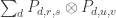


Now we’re trying to express the identity as a small linear combination of these convolution operators, so we can turn the problem into a one-dimensional problem: to write the function 

I am about 99% sure that if we could do that with a finite linear combination then we would have a proof of EDP. I used to think that “whatever works for finite should also work for infinite but with absolutely summable coefficients,” but it seems that this is wrong because even if the coefficients can be made very small, the functions themselves may be getting quite large in the norms we care about, so the convergence may be much too weak.
That does indeed seem to be the case here. If you convert the just-do-it argument above into an argument to express
Let me just elaborate on the remark that this problem can be solved directly by means of a just-do-it argument. I won’t give the full argument, but I’ll just point out that for each rational 


What is not so good about it is that the 

Thinking slightly further about this, I see that what I said above about pointwise convergence was a bit too pessimistic: for example, we can easily organize for the convergence to be uniform. And indeed, if we think of
Rational numbers sort of repel each other, so if we’ve devised 


What that boils down to is that this kind of greedy keep-away-from-everything-else approach doesn’t give us any kind of useful convergence, which we need if we are to get the averaging argument to work. I realize that I haven’t been too clear about what kind of convergence would work, but there is one kind that is definitely OK, and that is if we have a finite linear combination. So let me now ask a completely precise question.
A sufficient (I’m almost sure) condition for EDP
Let 


Summary.
In this post I have been looking at the representation-of-diagonals approach over the rationals with the extra symmetry constraint that the HAP products are all of the form 

Thinking through what this means, we find that we can reformulate the problem and obtain the question asked in the previous section.
Where next for EDP?
To finish, I’d like to ask if anyone has views about how they would like the EDP project to proceed. We are in uncharted waters at the moment: we have a project that started with a burst of activity — in fact it was sustained enough to count as more than just a burst — but now it has slowed right down and I’m not sure it will ever regain anything like its earlier intensity. And yet I myself am still enthusiastic about it, and perhaps I’m not alone in that.
My question is what should happen if it turns out that there are only two or three people, or even just one, who feel like working on the problem. In that case, there are various options. We could simply continue to post comments on this blog and not worry if there are very few participants or if the rate of posting is small. Or we could move the project to a different phase, more like a normal collaboration, with longer periods of private thought, but from time to time write comments or posts to make sure that any important developments are kept public (so that, in particular, anyone who wanted to join in would be free to do so). Or we could turn the project into a completely conventional collaboration, always with the understanding that the author of the eventual paper would be D. H. J. Polymath. And that’s not quite the most conventional it could go. The final possibility would be to close the project altogether, write a paper summarizing all the partial results, and then “free up” the problem for anyone who wants to think about it privately — if they used any of Polymath’s ideas they could simply refer to the paper that contained those ideas.
I think I favour keeping the project going as a Polymath project but with longer periods of private thought, but I don’t favour this strongly enough that I couldn’t be persuaded to change my mind if others feel differently. If that is the way we go, then my final question is, are there people out there who would like to be part of a small group of reasonably dedicated participants, or am I on my own now?

September 3, 2010 at 8:45 pm |
I have made some progress on the graph theoretic approach but I have not written anything up because of lack of time. If your offer still stands to make a post outlining how a new approach would work I’d be willing to give it a go, but I’m not sure if that would inject any new energy.
September 3, 2010 at 9:01 pm |
I think keeping this as a polymath project with longer periods of thought is a reasonable way to continue. This project interests me but I don’t know how much I can contribute to it. I don’t know what other people’s level of contribution will be.
September 3, 2010 at 9:36 pm |
[…] Polymath5 By kristalcantwell There is a new thread for Polymath5 here. […]
September 4, 2010 at 9:37 am |
Since now it is the reverse from the beginning (when the rate of comments was driving the rate of new posts), there’s the new possibility of setting a fairly regular pace for new posts, like a real weekly workgroup. This might then have a beneficial effect on the commitment of the participants (allowing it to fit in one’s regular schedule).
So the transition to a polymath with longer periods of thought seems very natural. Also, keeping this as a polymath would allow students to still learn from your thought process, and any non-working ideas to be recorded. (I’m probably not able to contribute anything apart from a little numerics and plots, but would be very happy to learn how the problem can be solved).
September 4, 2010 at 11:08 am |
I don’t know whether everyone who wants to express an opinion about this has done so, but I’m not getting the impression that people are falling over themselves to participate fully, and I’m also getting the impression that if that is the case, then people wouldn’t mind if I worked privately but wrote regular posts to say how I was getting on and give details about any new thoughts I might have had — always on the understanding that anybody who wanted to contribute could at any stage join in, and that if suddenly four or five people became enthusiastic then the collaboration would revert to the old style of working.
Incidentally, I find that one of the good things about Polymath that is quite independent of the number of people participating is that it forces you to make your thoughts clear enough to be explained to other people. So even a monomath project has some value.
One other thing I wanted to say is that I sometimes worry that when I write a post such as the one above that contains some calculations, people are a little bit put off by the calculations and feel that to contribute they would need to invest a large amount of effort just to understand what on earth I was saying. I tried to write the last few sections so that one could understand those and ignore the rest of the post, but I realize that there is more that I could have said. So I’d like to ask whether this is partly the case. Should I be trying to write something like a paper, with precise results (along the lines of “If we could do A then we could do B”), precise conjectures, and plenty of chat in between? I’m tempted to do that anyway, because I think it could easily be modified to form part of whatever paper results from the project. (I’m assuming that there will be some kind of paper, whether or not the problem is solved.)
September 4, 2010 at 3:51 pm
Yes, I think it would be very interesting and useful to have “something like a paper” about where exactly you currently are and what the next steps ought to be.
September 5, 2010 at 7:20 pm
I’m still interested in the project but I haven’t had much time to devote to it lately.
September 5, 2010 at 8:03 pm
I’m now preparing a post in which I hope to give a rigorous proof of why the decomposition discussed above would imply EDP if it existed for arbitrarily small I think we now have a genuinely new avenue to explore, and that just like most of the other avenues it lends itself to a mixture of theoretical and numerical investigations.
September 4, 2010 at 11:55 am |
Do we have such a finite decomposition of for any
  ?
?
September 4, 2010 at 12:46 pm
That’s a good question, to which I do not know the answer. It fits well with something I was thinking a little earlier, which is that there might be more hope of finding interesting decompositions with this one-dimensional problem than there was with the earlier two-dimensional problem.
The general problem is to represent one vector as a linear combination
  with
with  as small as possible. I haven’t quite worked out what that is — is it simply a linear programming problem? Or is it a dual linear programming problem? In particular, is it a problem for which there are very efficient packages out there waiting to be used? If so, then perhaps there is a hope of using a mixture of theory and experiment to prove a lower bound for discrepancy that’s better than our current record of 3. But even if we didn’t manage that, I think any decomposition with
  would be interesting. (I don’t rule out, however, that there is some fairly simple decomposition that gives something like
  and that the real interest starts below that.)
One other thing I’m not quite clear about is the extent to which examples such as the sequences of length 1124 translate into constraints on the decompositions one can hope to find. The reason for that is that passing to the rationals means that there isn’t a completely instant quantitative translation from one problem to the other. In principle, that might be good news as it might mean that in order to obtain a decomposition with, say, one would not have to look at functions with huge supports.
September 4, 2010 at 2:29 pm
It looks like a convex optimization problem with linear constraints, which should be solvable quite efficiently – although the number of variables is large (of order if we consider all subintervals of
  ). I’ll have a go at it with some small
  and see what happens …
September 4, 2010 at 3:22 pm
I think one can get away with just variables by considering functions just of the form
  The reason is that we have a sort of polarization identity here. (I think I made the same point but in a different context somewhere in the post above.) First of all, note that the value of
  at
at  is the same as the value of
  at
at  Therefore, given any decomposition of
  we can replace each
  by
by  and obtain a symmetric decomposition: that is, one that always gives the same coefficient to
  that it gives to
Next, notice that, equating sets with their characteristic functions,![[r,s]\times[u,v]+[u,v]\times[r,s]](https://s0.wp.com/latex.php?latex=%5Br%2Cs%5D%5Ctimes%5Bu%2Cv%5D%2B%5Bu%2Cv%5D%5Ctimes%5Br%2Cs%5D&bg=ffffff&fg=333333&s=0&c=20201002) is equal to
is equal to
To convert these functions into functions defined on we just think of each point of
  as a rational number and sum up. (By “sum up” I mean that for a rational like 2/3 we would add up the values at
  etc.) Therefore,
  is equal to
Thus, if we can decompose into functions of the form
  with sum of coefficients at most
  then we can decompose into functions of the form
  with sum of coefficients at most
It’s not clear to me whether for small the gain you get from having only
  variables is more or less important than that factor 4. But it certainly allows you to look at much larger
  so seems worth trying — after all, if it is possible to decompose
  into functions of the form
  with a reasonably small constant
  then one has a stronger result.
September 4, 2010 at 9:19 pm
Ah yes, that looks useful.
In fact the problem can be expressed as a linear optimization problem, at the expense of doubling the number of variables and adding some constraints: one just has to write , with
  , and minimize
  .
.
I’ve written a program in Python using the ‘cvxopt’ package to solve this. For a first attempt I allowed all possible pairs of intervals. It turns out that is achievable, using subsets of
  . The program came up with the solution:
  ,
,  ,
,  ,
,  , and
, and  (to abbreviate your notation slightly). It’s easy to check that this works.
I’ll do some more investigation …
September 4, 2010 at 9:22 pm
Sorry, I meant to write:
September 4, 2010 at 10:44 pm
Simple as it is, I find that example rather encouraging because it genuinely relies on the new symmetric set-up, in the sense that the function is not supported on the diagonal of
I suppose one should check whether a tensor-power trick can be used to convert this example into one that gives you a constant for arbitrary
  It would be a bit of a miracle if it did.
Hmm … I can’t really do this in my head, but it feels as though the answer is that it doesn’t, because a product of HAPs is a multidimensional HAP. But I may check this just in case something can be got to work.
Hmm again … can one do anything by taking the kth multiplicative convolution power of both sides of your identity? The right-hand side would not immediately be of the right form, but it’s not instantly clear to me that it can’t be decomposed into something of the right form. We would have terms, each multiplied by
  so we would need to find a way of decomposing each term into functions of the desired form with coefficients adding up to significantly less than
I’m putting that idea up in an old-style Polymath spirit — I’m not sure when I’ll be able to get round to thinking about it properly.
September 5, 2010 at 7:54 am
A few more data. Optimizing over all possible pairs of intervals, new records for are set at:
  (
( ),
),  (
( ),
),  (
( ),
),  (
( ),
),  (
( ).
).
Restricting to symmetric rectangles , we first attain
  at
at  . The solution here is:
  ,
,  ,
,  ,
,  ,
,  ,
,  , and
, and
where is shorthand for
  .
.
This attains . The next record-breaker for the symmetric case is
  , where we attain
  , with a combination of
  intervals each with coefficient
  .
.
September 5, 2010 at 8:29 am
… And the next is , where we attain
  , with a combination of
  intervals each with coefficient
  .
.
And the next is , where we attain
  , with a combination of
  intervals each with coefficient
  . For the record:
September 5, 2010 at 9:30 am
Hmm, there’s a pattern in that last decomposition. It’s:
No time to think more about this now, but it seems quite encouraging …
September 5, 2010 at 12:31 pm
I find the mere existence of these decompositions, whether patterned or not (though obviously patterns dangle in front of us the hope of generalization), pretty encouraging, though at this stage it’s not clear how encouraging they are. One thing I’m also finding is that, despite the appeal of having a 1D formulation, it’s perhaps easier to go back to the (equivalent) 2D set-up with lines in What I mean is that if we want to check that a decomposition
  works, then the easiest way of doing so (by hand, that is) is to look at the function
  and check that the sum along the main diagonal is 1 and the sum along all other lines through the origin is 0.
What I like about this is that in a certain sense it is strictly easier than what we were trying to do before. That is, before, we were trying to represent a diagonal as a linear combination of HAP products. Now all we need is that if you stand at the origin and do a sort of scan, it looks as though you have a diagonal matrix, even though in fact you may not. Another way of putting that is that you have lines going through the origin as test functions and if the inner product of with any one of those lines is what it would be if you had a diagonal matrix, then you count the decomposition as being OK. And that’s a lot weaker than requiring the decomposition to give you a diagonal matrix.
What I’ll do when I get the chance, unless you’ve already done so by then, is examine that pattern and see if it can be generalized. I think it is no coincidence that the record occurred at a nice smooth number like 60: if you have pairs where
where  and
and  are large primes, then they are hard to deal with, but the interval
 ![[54,60]](https://s0.wp.com/latex.php?latex=%5B54%2C60%5D&bg=ffffff&fg=333333&s=0&c=20201002) is full of smooth numbers. (OK there’s a bit of a problem with 59, but the contribution from
is full of smooth numbers. (OK there’s a bit of a problem with 59, but the contribution from ![[59,60]](https://s0.wp.com/latex.php?latex=%5B59%2C60%5D&bg=ffffff&fg=333333&s=0&c=20201002) deals with that.)
deals with that.)
September 5, 2010 at 12:56 pm |
Alec, as you’ve probably worked out in the meantime for yourself, this idea brings us down to . Why? Take any large natural number
  , set
, set  , and note that
  , where
 ![P_r=[n/r-1, n/r]](https://s0.wp.com/latex.php?latex=P_r%3D%5Bn%2Fr-1%2C+n%2Fr%5D&bg=ffffff&fg=333333&s=0&c=20201002) for
for  ,
, ![Q=[n-m, n-1]](https://s0.wp.com/latex.php?latex=Q%3D%5Bn-m%2C+n-1%5D&bg=ffffff&fg=333333&s=0&c=20201002) and
and ![R=[n-m, n]](https://s0.wp.com/latex.php?latex=R%3D%5Bn-m%2C+n%5D&bg=ffffff&fg=333333&s=0&c=20201002) . This yields a value of
. This yields a value of  for
for  , which, of course, tends to
  as
as  goes to infinity.
September 7, 2010 at 10:02 am
Christian, I’ve just found this comment of yours amongst my spam. I’ve no idea why it went there as it didn’t seem to have any obvious spam-like features, so apologies for that.
One other small remark is that if you want the TeX to compile you have to write the word “latex” immediately after the dollar sign. For instance, to produce I would write “$***** \int_0^1f(x)dx$” except that instead of “*****” I would write “latex”. I have edited your comment by inserting the “latex”s.
September 7, 2010 at 11:32 am
Tim, many thanks for editing the formulae, and for the explanation of how to do so myself in the future. The following equation is just meant as “experiment” without relevance to EDP:
September 5, 2010 at 1:40 pm |
Small remark: Alec’s pattern is interesting, but it’s not clear how to generalize it so as to decrease . Since a small
  means
means  , and since
  governs the number of intervals while
  is the number of times we hit the diagonal (if I understood correctly), then somehow we should have “not many” intervals. So I’m not sure what to do with the sum of many small intervals in Alec’s example (at least it shouldn’t grow too fast as
  decreases).
September 5, 2010 at 3:20 pm
I’m not sure I fully follow what you are saying, but I agree with you to the extent that it looks very unlikely that one could solve the problem with one big interval that is cancelled out, except on the diagonal, by lots of small ones.
September 5, 2010 at 4:17 pm
Let me try to put what you say in my own words, because I’m not sure I know what you mean by and
and  Suppose we have intervals
  and coefficients
  (
( ) such that
  sums to zero along every line with gradient not equal to 1. What value of
  does it give us? Well, the sum along the main diagonal is
  and the sum of the absolute values of the coefficients is
  So we get
  In the special case where each
  is
is  we get
  To make that more transparent, if the sum is
  then we get
  So we want a significant imbalance in the sizes of the
  and
and 
Another necessary condition is that the sum of off the diagonal is zero. (To see this, just sum the sums over all non-diagonal lines.) In the case of the
  and
and  this tells us that
  So, roughly speaking, we want the squares of the sizes of the negatively counted intervals and the positively counted intervals to be well balanced, but the sizes themselves not to be well balanced.
A small thought is that this puts a number-theoretic constraint on the sizes of the and
and  that could perhaps be used to narrow down the search, especially if one just searches for
  sums.
sums.
Going back to Thomas’s point, if we have one big interval, of size say, and try to cancel it out with lots of little intervals of bounded size, then it won’t work because we’ll need
  little intervals in order to get the off-diagonal sum equal to zero, and then we have
  and the imbalance in the sums of the sizes of the intervals equal to
  so we will never do better than some absolute constant for
  But if our little intervals have size
  say, then we have roughly
  of them, and an imbalance of more like
  So that gives us
The point I’m making here is that for all we know it might be possible to prove EDP by finding one big interval and cancelling it out using lots of small intervals, provided only that the sizes of the small intervals tend to infinity. (I call them small because I don’t care if they have size where
where  is the size of the big interval.)
September 5, 2010 at 5:13 pm
Sorry for the sloppy notation and poor wording, and thank you for these details, and the other constraints. Yes that’s what I had in mind: the interplay between the number of intervals and the behaviour
  on the diagonal.
September 5, 2010 at 8:20 pm
Yes, the pattern only generalizes in an obvious way to the extent of giving us arbitraily close to
  . Indeed, for any
  , we can write
since each of the off-diagonal terms in the blocks is cancelled by a term in the difference between the two large blocks.
Perhaps this merely confirms Tim’s suggestion that the problem might only become interesting for or something. But it seems worth asking whether we can generalize the pattern further to give us
  by taking a sum of blocks of size
  plus a small number of larger blocks – although there may be a simple reason why that can’t work.
September 5, 2010 at 2:55 pm |
At some point I also thought of writing up a post going back to some earlier avenues and questions. The Decomposition approach and related SDP and LP is very nice and it has several features that makes it the most promising, but sometime down the road it will be useful to think or write down some older approaches and problems. In any case, keeping this project open for several additional months seems preferable to me.
September 5, 2010 at 3:26 pm
Any efforts in that direction would be greatly appreciated. For instance, one thing that I would be sorry not to return to is the behaviour of multiplicative functions produced by various greedy and not so greedy algorithms. There seemed to be some very interesting phenomena there that we failed to understand even heuristically.
I haven’t pinned this down 100% and have therefore not said too much about it, but on a couple of occasions I have had thoughts related to decompositions that seem to lead either to the very nice observation that Terry made concerning reducing the problem to one about multiplicative functions or to something very like it. So it may be that there will be some kind of convergence of the different approaches. Another idea that it would be good to resurrect is the one that I know interests you, and interest me too — of trying to show that EDP is true for wide classes of sequences, such as sequences that do not correlate with character-like functions. A partial result like that, especially if it could be proved with a better bound than can be expected for EDP in general, could be very enlightening.
September 5, 2010 at 11:24 pm |
Just to summarize what Alec obtains in this comment and the build-up to it, we now have a method that’s in retrospect fairly simple for getting a decomposition that will get us down to The idea is this. You choose
  that is divisible by all of
  You then take the difference between the square
 ![[N-k,N]^2](https://s0.wp.com/latex.php?latex=%5BN-k%2CN%5D%5E2&bg=ffffff&fg=333333&s=0&c=20201002) and the square
and the square ![[N-k,N-1]^2.](https://s0.wp.com/latex.php?latex=%5BN-k%2CN-1%5D%5E2.&bg=ffffff&fg=333333&s=0&c=20201002) This gives you all points of the form
This gives you all points of the form  or
or  with
with  We now want to cancel out all of those except the point
  To cancel out the points
  and
and  you use the square
 ![[N/j-1,N/j]^2.](https://s0.wp.com/latex.php?latex=%5BN%2Fj-1%2CN%2Fj%5D%5E2.&bg=ffffff&fg=333333&s=0&c=20201002) The reason that works is that the line through the point
The reason that works is that the line through the point  also goes through the point
  and it goes through none of the other points that we have left. And similarly for the reflected line on the other side of the diagonal. So we end up doing all the calculations we wanted to do.
As a little experiment, let’s think what would happen if we took the square![[N/j-2,N]^2](https://s0.wp.com/latex.php?latex=%5BN%2Fj-2%2CN%5D%5E2&bg=ffffff&fg=333333&s=0&c=20201002) instead. Now we have a few more lines going through points in the square. The points above the main diagonal are
instead. Now we have a few more lines going through points in the square. The points above the main diagonal are 
 and
and  Multiplying all these through by
  gives us the points
 and
and 
Ah, that itself isn’t ideal, but what if is even and we take the square
 ![[N/2-k/2,N/2]^2](https://s0.wp.com/latex.php?latex=%5BN%2F2-k%2F2%2CN%2F2%5D%5E2&bg=ffffff&fg=333333&s=0&c=20201002) and subtract the square
and subtract the square ![[N/2-k/2,N/2-1]^2](https://s0.wp.com/latex.php?latex=%5BN%2F2-k%2F2%2CN%2F2-1%5D%5E2&bg=ffffff&fg=333333&s=0&c=20201002) ? We can use that to knock out all points of the form
? We can use that to knock out all points of the form  with
with  even, I think. If we get rid of all the others in a trivial way, does that improve
  ? And if it does, can we continue along similar lines and get
  smaller still? I have to stop for the day, so I can’t think about this just yet.
September 6, 2010 at 8:16 am
Sorry, that obviously won’t improve on 1/2 because the bulk of the work is still done by intervals of length 2.
September 6, 2010 at 4:54 pm |
I’d like to mention an idea that I think is unlikely to work, but it feels like the next obvious thing to try after Alec’s construction. His construction works by taking what I like to think of as a sort of rotated-L-shaped “fly trap”![[N-k,N]^2-[N-k,N-1]^2](https://s0.wp.com/latex.php?latex=%5BN-k%2CN%5D%5E2-%5BN-k%2CN-1%5D%5E2&bg=ffffff&fg=333333&s=0&c=20201002) and making sure that exactly one fly gets caught in each place. A “fly” is a point in one of the other squares that flies out along a straight line that starts at the origin.
and making sure that exactly one fly gets caught in each place. A “fly” is a point in one of the other squares that flies out along a straight line that starts at the origin.
The “trivial” method of achieving this is to have exactly one fly (or rather, symmetric-about-diagonal pair of flies) per little square, and to make so big and smooth that we can find such a thing for every point of the form
  or
or  But that will never get us
  better than
  because we have so many squares of width 2. So we want a construction where most of the squares are significantly bigger.
What I’m wondering is whether we can keep the fly trap idea, but do it much more economically by trying to hit almost all points in the trap rather than all of them. The basic idea would be that we could take squares of unbounded size and use those to create enough flies to hit a proportion of the points in the trap, and then deal with the remaining points in a completely trivial way, knocking them out one by one. The trivial part would be uneconomical, but since the proportion of points belonging to the trivial part would be small, this wouldn’t matter.
To give a slightly more precise idea of how a fly trap might catch the flies from a larger square, let us consider a square![[r,s]^2](https://s0.wp.com/latex.php?latex=%5Br%2Cs%5D%5E2&bg=ffffff&fg=333333&s=0&c=20201002) where
where  is of unbounded size (but we can think of it as a very large constant) and much smaller than
Now let’s suppose that is divisible by every number from
  to
to  Then every point
 ![(a,b)\in[r,s]^2](https://s0.wp.com/latex.php?latex=%28a%2Cb%29%5Cin%5Br%2Cs%5D%5E2&bg=ffffff&fg=333333&s=0&c=20201002) with
with  has some multiple of the form
  with
with  and every point
 ![(a,b)\in[r,s]^2](https://s0.wp.com/latex.php?latex=%28a%2Cb%29%5Cin%5Br%2Cs%5D%5E2&bg=ffffff&fg=333333&s=0&c=20201002) with
with  has some multiple of the form
  with
with  These points belong to a “fly trap”, but the difference now is that the width of the fly trap is much bigger (as a function of
  ) than it was in Alec’s construction: in order for
  to be divisible by every number between
  and
and  it must be very much bigger than
  or
or  ; but the width of the trap is at least
  or thereabouts.
What this demonstrates is merely that it is possible for all the points in a rectangle of unbounded size to get caught in a fly trap. What it does not show is that we can use up more than a handful of points in the fly trap this way. My guess is that we can’t — that’s what I plan to think about next.
(General remark: I’m temporarily back in normal Polymath mode, since there is some interaction going on.)
September 7, 2010 at 6:59 am |
I agree that finding a decomposition with would be very interesting. Getting
  blocks to cancel seems to be much harder than with
  blocks!
Here’s just a tiny thought in that direction. Closely related to the decomposition
is the decomposition
If we add these two decompositions together, the pairs of terms![[\frac{N}{r} - 1, \frac{N}{r}]^2 + [\frac{N}{r}, \frac{N}{r} + 1]^2](https://s0.wp.com/latex.php?latex=%5B%5Cfrac%7BN%7D%7Br%7D+-+1%2C+%5Cfrac%7BN%7D%7Br%7D%5D%5E2+%2B+%5B%5Cfrac%7BN%7D%7Br%7D%2C+%5Cfrac%7BN%7D%7Br%7D+%2B+1%5D%5E2&bg=ffffff&fg=333333&s=0&c=20201002) fill all but two of the points of a
fill all but two of the points of a  square,
 ![[\frac{N}{r} - 1, \frac{N}{r} + 1]^2](https://s0.wp.com/latex.php?latex=%5B%5Cfrac%7BN%7D%7Br%7D+-+1%2C+%5Cfrac%7BN%7D%7Br%7D+%2B+1%5D%5E2&bg=ffffff&fg=333333&s=0&c=20201002) , with the middle one counted twice.
, with the middle one counted twice.
What if we try to form a decomposition with the sum
We’re left with the terms and
and  . But I can’t see how to construct a fly-trap to cancel these.
September 7, 2010 at 10:52 am |
One thought I had about fly traps is that we should expect them to be difficult to construct. To see what I mean by this, let’s imagine that we tried to create a fly trap out of a square![[r,s]^2.](https://s0.wp.com/latex.php?latex=%5Br%2Cs%5D%5E2.&bg=ffffff&fg=333333&s=0&c=20201002) If we just choose a fairly random pair of integers
If we just choose a fairly random pair of integers  and
and  (perhaps with
  not much bigger than
  ) then we can expect
 ![[r,s]^2](https://s0.wp.com/latex.php?latex=%5Br%2Cs%5D%5E2&bg=ffffff&fg=333333&s=0&c=20201002) to contain many pairs
to contain many pairs  of coprime integers, since there is a positive probability that two random integers are coprime. OK, they’re not quite random here because they are fairly close to each other, but I don’t think that makes a substantial difference. Indeed, if
  then they are guaranteed to be coprime, if
  and they are both odd then they are guaranteed to be coprime, and in general if
  and
and  is coprime to
  then they are guaranteed to be coprime. So it seems to me that if
  isn’t tiny then we get a rich supply of coprime pairs in the square
 ![[s-r]^2.](https://s0.wp.com/latex.php?latex=%5Bs-r%5D%5E2.&bg=ffffff&fg=333333&s=0&c=20201002)
The problem with coprime pairs is that there is nothing for them to trap, since each one is the first integer point along the line from the origin.
So how might we create a nice big and fairly simple rectilinear region that does not contain lots of coprime pairs? So far we have used the following simple technique: find a very smooth and simply take an inverted L shape with its corner at
  Each point in that shape will have a coordinate equal to
  and since
  has lots of small factors, it is quite hard to be coprime to
Now suppose we wanted to thicken up that inverted L shape a bit. What we would ideally like is an interval![[N,N+r]](https://s0.wp.com/latex.php?latex=%5BN%2CN%2Br%5D&bg=ffffff&fg=333333&s=0&c=20201002) such that most of the points in it are smooth enough to have common factors with almost all positive integers. But that gets us into worrying ABC territory — we can expect it to be difficult to cram lots of highly smooth integers into a small interval. (I’ve now looked up the ABC conjecture and I’m not sure after all that it is relevant. But I still don’t see how to get an interval that’s full of integers each with lots of distinct small prime factors, which is what would be needed for this to work.)
such that most of the points in it are smooth enough to have common factors with almost all positive integers. But that gets us into worrying ABC territory — we can expect it to be difficult to cram lots of highly smooth integers into a small interval. (I’ve now looked up the ABC conjecture and I’m not sure after all that it is relevant. But I still don’t see how to get an interval that’s full of integers each with lots of distinct small prime factors, which is what would be needed for this to work.)
A thickened inverted L can be thought of as a whole lot of inverted Ls all pushed together. It has the advantage that it can be represented very efficiently in terms of rectangles, but it’s not clear that we need such extreme efficiency, so perhaps a better idea is not to insist that they are all pushed together. That avoids the number-theoretic problems just discussed. So the plan would be something like this. First choose some largish positive integer Next, find a number of large integers
  all around the same size, and all of them products of some of the first
  primes (not necessarily avoiding multiplicity). Since the sum of the reciprocals of the primes diverges, we can choose
  large enough that
  is very small, and if we do that then even if
  is a random subset of
  then
then  will be small. So in that way we have a rich supply of integers that are of size somewhere around
  and that are coprime to only a very small proportion of other integers.
We could use these to create a sort of reception committee of fly traps. (The phrase “reception committee” is chosen for the benefit of Cambridge backgammon fans.)
What I would be hoping for here is something like this. Suppose we now take a smallish square![[u,v]^2.](https://s0.wp.com/latex.php?latex=%5Bu%2Cv%5D%5E2.&bg=ffffff&fg=333333&s=0&c=20201002) We would like it to cancel out some of the points in all those fly traps. Let’s consider a typical point
We would like it to cancel out some of the points in all those fly traps. Let’s consider a typical point ![(a,b)\in[u,v]^2](https://s0.wp.com/latex.php?latex=%28a%2Cb%29%5Cin%5Bu%2Cv%5D%5E2&bg=ffffff&fg=333333&s=0&c=20201002) and let us suppose that
and let us suppose that  and
and  are of roughly the same size. Then as we take multiples of
  we will expect them to hit any given fly trap with probability roughly
  So we might hope that if we have about
  fly traps, then we will typically expect to hit one and only one of them. But even better might be to have
  fly traps for some large constant
  so that concentration of measure could kick in and tell us that with high probability we will hit about
  of the fly traps. What I’m hoping for here is that we could use probabilistic methods: we choose a bunch of random small squares
 ![[u,v]^2](https://s0.wp.com/latex.php?latex=%5Bu%2Cv%5D%5E2&bg=ffffff&fg=333333&s=0&c=20201002) and argue that the points in the fly traps mostly get hit about the same number of times. (I am very far from sure that this is correct, since it ought to depend on “how non-coprime” the coordinates of the points in the flytraps are. But perhaps some Erdős-Kac type phenomenon would tell us that most points were about the same in this respect.)
and argue that the points in the fly traps mostly get hit about the same number of times. (I am very far from sure that this is correct, since it ought to depend on “how non-coprime” the coordinates of the points in the flytraps are. But perhaps some Erdős-Kac type phenomenon would tell us that most points were about the same in this respect.)
The general idea here would be to hit most of the points in the fly traps about the same number of times, and then divide through the small squares by that number and subtract. This would leave us with an approximate cancellation, and the remaining error could be mopped up with a trivial decomposition.
This is all a bit of a fantasy at the moment, but I think it’s the kind of thing we need to try.
September 7, 2010 at 12:37 pm |
Here are a few more thoughts about the reception committee of fly traps idea.
I won’t give the full details, but at first I thought I had an argument to show that it couldn’t work, but then I realized that it might just be possible, though I am at the moment ignoring certain aspects of the problem that are probably important. To be precise, I am ignoring the question of whether we can find sufficiently many smooth large integers that are all reasonably close to each other.
The parameters we need to choose are the number of inverted Ls and their lengths. (To be clear, let us define the length of the set of integer points along the lines from to
to  and
and  to be
to be  And let’s call that set
  After a bit of experimenting, I realized that we need really rather a lot of layers to the fly trap. Let me try to explain roughly why. Given a point in
  that is not on the main diagonal, it is within
  of the point
  so there cannot be any positive integer points on the line joining that point to the origin with
  coordinate less than
  (since then it would be within less than 1 of the main diagonal). But that means that the probability of a multiple of a point in one of the small squares hitting a given inverted
  can be at most
  which means that for the argument to work we will need at least
  layers.
I won’t say more, but those are the kinds of calculations that underlie the details of the following suggestion. I would like to choose roughly inverted Ls of length roughly
  between
  and
and  I would like them all to be of the form
  with each
  having enough small prime factors for almost all positive integers to have common factors with
  Note that each inverted L can be created with a contribution of 2 to the sum of the absolute values of the coefficients, so so far we have got up to
  for this.
Now for the cancelling part. This we shall create as a whole lot of fairly randomly chosen squares![[r_i,s_i]^2](https://s0.wp.com/latex.php?latex=%5Br_i%2Cs_i%5D%5E2&bg=ffffff&fg=333333&s=0&c=20201002) where each
where each  has order of magnitude
  and each
  has order of magnitude
  That means that each square contains roughly
  points off the diagonal, so in order to do the cancellation, we need about
  of them. (In practice, I would expect to take more like
  of them and divide them all by
  , just to smooth things out a bit.) If the probabilistic heuristic works, then each point will … oh dear, I’ve made a mistake.
My mistake is that if we have squares of width
  then we’ll be forced to go all the way up to
  which means that for the probabilistic heuristic to work we’ll need
  layers. Let me go back and do a few more calculations.
September 7, 2010 at 1:02 pm |
This deserves a new comment. Let’s suppose that we have inverted Ls of width
  between
  and
and  Then the number of points we have to cancel is
  (I’m stating everything up to an absolute constant.) For the probabilistic heuristic to work, we need the points we use to do the cancelling to have coordinates bounded above by
  (or else the probability that they hit one of the layers of the reception committee is significantly less than 1 and we end up with lots of uncancelled points). But the number of points with coordinates bounded above by
  that are close enough to the diagonal to cancel any of the points in the reception committee is at most
  So we need
  to be at least
  which implies that we need
  to be at least
  But that’s a problem because we now have so many points we want to cancel that we are forced to have the little squares centred at points that are higher up than
It’s just conceivable that we can get round this by showing that if we choose our inverted Ls to be at fairly smooth heights, then the probability of hitting them is significantly larger. (There is some plausibility to this: for instance, if you go to the opposite extreme and take them at prime height then you cannot hit them.) However, the question in my mind then is whether this increase in probability is enough to compensate for the fact that there are fewer layers.
September 7, 2010 at 2:16 pm |
There are all sorts of difficulties emerging with this basic idea, though I still don’t have a strong feeling about whether they are completely insuperable. Another thought is that if we are using a fairly random selection of small squares, then we will want the points in the layers to have roughly the same size highest common factor. Why? Well, if the highest common factor of
  and
and  is
is  then the number of positive integer points on the line from
  to
to  is
is  (the number of multiples of
  up to
up to  ). And if we are choosing the squares randomly, then we’ll expect to hit each positive integer point with about the same probability.
Can we find integers such that for most small
  the highest common factor of
  and
and  is about the same? It doesn’t sound very likely, but let’s think about it by considering the number
  and asking how we expect the highest common factor of
  with a random integer
  to be distributed.
The log of the highest common factor will be where
where  with probability
  The expectation of this tends to infinity with
  If I’m not much mistaken, the variance is roughly the same size as the expectation, so the standard deviation, as a fraction of the mean, should tend to zero. So it looks as though there is some hope that the function is reasonably concentrated for nice smooth
Except that I’m forgetting that I started by taking logs. So in order for the hcf itself to be reasonably concentrated, we would need the log of the hcf to be highly concentrated. In fact, I don’t believe that the hcf is concentrated at all: for example, if is even, then I’d expect that conditioning on
  being even would significantly increase the expected hcf with
I’m not sure where that leaves us. I’m having a lot of difficulty thinking of even a vaguely plausible way of building a decomposition using lots of inverted Ls. But I don’t have much of an idea of a theoretical statement that expresses this difficulty, or of what other construction methods one might imagine using.
September 7, 2010 at 4:23 pm |
I have a more general idea, but I’m far from sure that it works. It’s again motivated by the thought that we might be able to get somewhere by a clever probabilistic approach that gives a good approximation to a decomposition followed by a crude determinisitc approach to sweep up the remaining error.
Here’s the thought. If we’re going to choose things randomly, then we will tend to hit lines with gradients that are rationals with small numerator and denominator more frequently than lines with gradients that are rationals with large numerator and denominator. Indeed, we will tend to hit a line with a frequency that’s proportional to the density of integer points along that line. Let’s quickly work out what that density is, on the assumption that the gradient of the line is fairly close to 1. If the gradient is where this fraction is in its lowest terms, then the integer points are
  and so on. So they occur with frequency proportional to
If we have an arbitrary point and
and  when written in its lowest terms, that tells us that a randomish set of density
  will hit the line containing
  with frequency about
This suggests that we might be able to do something by constructing two randomish sets of density in different ways, one that hits the diagonal a lot and the other that does not hit it nearly so much. Then we could subtract the two and get a big trace and not all that big a sum of coefficients.
For instance, one set could be made out of quite a lot of fairly long inverted Ls, arranged reasonably randomly, but based at points that are smooth enough that there aren’t too many coprime pairs. Then the other set could be made out of smallish squares that are on average somewhat nearer the origin.
This sounds a bit like what I was suggestion before, but there are differences. One is that we would no longer be trying, hopelessly, to make all the hcfs about the same — instead, we would just go with the natural distribution that assigns more weight to points that are on dense lines. Another is that we wouldn’t be too hung up about whether the squares and the inverted Ls overlapped. We’d just be trying to produce the same natural distribution in two different ways.
September 7, 2010 at 5:48 pm
Roughly speaking, what I think we’d be trying to show is that a random fraction for smallish
  and pretty smooth
  is distributed very similarly to a random fraction
  where
where  and
and  are close to each other and quite a lot smaller than
September 7, 2010 at 10:47 pm |
Let me try to think in real time, so to speak, about whether there is any hope of getting a probability distribution in two different ways.
Suppose that (unnecessarily specifically) is a product of a random subset of the primes
  And suppose also that
  is a random integer between
  and
and  where
where  is pretty large but quite a lot smaller than
  Then what is the distribution of
  or equivalently of
  ?
?
If is pretty large and random, then it will be divisible by
  with probability
  so we’ll expect it to be divisible by about
  of the
  So we should end up with a fraction
  where
where  is something like a random product of
  of the primes
  and
and  is coprime to
That’s not quite what I want. Let’s think about it the other way. Suppose I have a point such that
  and
and  have no common factors. What is the probability that some multiple of
  is of the form
  (assuming that
  ). We need
  to be a multiple of
  and then we are guaranteed to be OK provided only that
  is not too big.
But if we are choosing our not to be a random integer but a random pretty smooth integer, then the probability that it is a multiple of
  depends a lot on the prime factorization of
I have to stop for now, but it’s not a bad moment to do so as things are starting to look difficult again.
September 8, 2010 at 10:36 am |
In this comment I’m going to try to explain the idea behind my previous comment a bit more coherently.
Suppose we have a small “wedge” about the main diagonal. By that I mean that we take some small and look at all positive integer points
  such that
  lies between
  and
and  and both
  and
and  are at most
  Almost certainly we will want
  to tend to zero with
  — at any rate, we definitely allow this. Let us call this wedge
With each point in
in  we associate the rational number
  which is the gradient of the line from
  to that point. Also, with any subset
  we associate the function
  defined on the positive rationals, where
  is the number of ways of writing
  as
as  with
with  (We can think of this as a projection on to the line
  where we project each point along the line that joins it to the origin. We could also imagine that we are standing at the origin with a kind of scanner that can tell us, for any direction we point the machine in, how many points of
  there are in that direction.)
More generally, we can apply the above projection to multisets and functions. This will sometimes be useful. For instance, if I take a sum of sets of the form![[r,s]^2](https://s0.wp.com/latex.php?latex=%5Br%2Cs%5D%5E2&bg=ffffff&fg=333333&s=0&c=20201002) that are not necessarily disjoint, then I can simply sum up their projections. Just to be explicit, suppose I have a function
that are not necessarily disjoint, then I can simply sum up their projections. Just to be explicit, suppose I have a function  defined on
  Then I’ll define
  to be
to be 
What I’d like to do now, though I don’t have a strong feeling that it’s actually possible, is create some projected function in two ways, one using a function made out of a sum of small squares and one using a function
  made out of big squares.
I’m prepared to tolerate a certain amount of inaccuracy — precisely how much I haven’t worked out.
Here is the kind of way that one might hope to do this. The first way is to take all intervals![[r,s]](https://s0.wp.com/latex.php?latex=%5Br%2Cs%5D&bg=ffffff&fg=333333&s=0&c=20201002) such that
such that  and
and  where
where  for some large constant
  (Our eventual aim is to prove that the discrepancy of every
  sequence is at least as big as any constant you like to choose. So the bigger the discrepancy you want to prove, the bigger this
  will have to be.) If we now sum up the functions
 ![[r,s]](https://s0.wp.com/latex.php?latex=%5Br%2Cs%5D&bg=ffffff&fg=333333&s=0&c=20201002) to obtain a function
to obtain a function  (defined on
  ) and project, we will obtain a function
  such that
  is closely related to
  More precisely, there are two factors at work here: the further the line is from the main diagonal, the less it will be hit by the squares that are working their way up, and the more points there are on the line, the more that line will be hit. I haven’t worked out carefully what function that ought to lead to.
Now let us think how we might hope to create roughly the same projected function using larger squares. The basic idea would be to use quite a lot of inverted Ls, but put them (on average) further up the diagonal. Before I say more about how that might be done, let me explain why it would be good if we could do it.
Suppose, just to idealize a bit, that we managed to get exactly the same distribution, once using a sum of squares![[r,s]^2](https://s0.wp.com/latex.php?latex=%5Br%2Cs%5D%5E2&bg=ffffff&fg=333333&s=0&c=20201002) with
with  typically of size about
  and once using a sum of inverted Ls of length typically around
  Suppose also that the number of squares used is
  Then the number of off-diagonal elements of the squares would be around
  so the number of inverted Ls needed would be about
  That means that the sum of coefficients would be proportional to $latexs TM/C$ (since
  would be bigger than
  ). The sum along the diagonal would be
  or about
  The ratio of the two would be about
  so we would obtain a
  of about
  and a discrepancy bound of about
But is there any hope of doing this? The most obvious obstacle is that if you take the inverted L (defined to be the set of all points
  such that one of
  and
and  equals
  and the other is between
  and
and  ) then for every point
  such that
  and
and  are coprime, you get a line that will not intersect any of the squares. So it is very important that we do not have many of these coprime pairs.
But if we make sure that has a reasonable number of small prime factors (large enough for the reciprocals of those factors to have a sum that’s distinctly bigger than 1) then this will happen for only a small fraction of
  (I’ve just noticed that I’ve overused
  — once for the size of the wedge and once for the position of an inverted L. Let’s say that we are living inside the wedge
  rather than the wedge
  ) So then a typical point in
  will belong to a line that contains other points significantly nearer to the origin.
The real question is whether we can choose a bunch of different in such a way that these other points will be distributed in roughly the same way as if we choose a random square that just fits into
  and then a random point in that square. I don’t have an answer to that for now, but the main purpose of this comment was to ask the question as precisely as I could.
September 8, 2010 at 9:32 pm |
I’m not sure how to search directly for decompositions with , so in an attempt to discover some new patterns I tried forcing the decomposition (still restricted to symmetric rectangles
  ) not to have too many
  blocks in it. I’m not sure how useful the results are, but will post them here in case they give inspiration to anyone else.
First, I searched for the best solution with that contained no blocks
 ![[a, a+1]^2](https://s0.wp.com/latex.php?latex=%5Ba%2C+a%2B1%5D%5E2&bg=ffffff&fg=333333&s=0&c=20201002) with
with  . The best
  one can obtain with this constraint is just over 1, with the decomposition illustrated here.
Then, I searched for the best solution with and the sum of the absolute values of the coefficients of the
  blocks no greater than
  . This time one can get
  , with the decomposition illustrated here.
The patterns are quite similar, with blocks tending to be situated around divisors of
  . They still rely on the basic fly-trap construction. Each fly trap is ‘smoothed’ with a
  square in the middle, meaning that it has a ‘cost’ of 3 (in terms of coefficients) for a ‘benefit’ of 1 (the spare point of the
  square). Of course, the rest of the benefit has to come from the cancellations in the arms.
September 9, 2010 at 8:51 am
Alec, if you can modify your program to print the linear program to a fil in e.g. the MPS file format I can try to solve a few larger cases as well. That could be interesting for both the basic linear program and the restricted versions.
September 9, 2010 at 9:16 am
One quite interesting feature of the decomposition you obtain is that in a sense it does what I was trying to do theoretically: it finds a decomposition that works pretty well and then gets rid of a bit of error in a crude way by adding those blocks (to deal with points like
  ). It’s weak evidence, but maybe it suggests that that kind of approach is on the right track.
September 9, 2010 at 10:15 am
Klas, I should be able to do that — I’ll have a go later today.
September 9, 2010 at 8:59 pm
I think everybody should be able to access this:
https://docs.google.com/leaf?id=0B9uiJt0wroYCYThjY2FkNDItMzlmNS00ZTU2LThkZTUtYmM0YTg1MjFhZDM0&hl=en_GB&authkey=COmAtvoL
Let me know if not.
It is a Python file. I’ve tried to explain the usage in the comments at the top and within the functions. You will need the ‘cvxopt’ module to run it (this is freely downloadable — I won’t post the link because that would make this message land in Tim’s moderation queue — it’s easy to find).
Anyone with Python and cvxopt installed can use this program to solve decomposition problems restricted to any set of rectangles of the form . More complex constraint options could be added.
You can also use it to output MPS files. Unfortunately, I haven’t myself managed to read from the resulting file using cvxopt’s tools, so I’m not very confident that this is working (the files it produces look reasonable, though). Klas, perhaps you can try it and let me know!
September 10, 2010 at 12:56 pm
I’ve just tried opening the MPS file produced by the Python program using the LPSolve IDE in Windows. It does open it, and solve it — impresively fast.
September 10, 2010 at 1:36 pm
I am aso trying the program out now. I’m first runnign the python program with cvxopt and later I’ll try out the mps-files with one or two of my other solvers.
Any opinions regarding what the most interesting cases to try here would be?
September 10, 2010 at 2:21 pm
Unfortunately I’m not computer literate enough to try the program out. But I am in the middle of writing a post that I hope will suggest promising ways of narrowing down the search for examples. It should be ready in the next hour or two.
September 10, 2010 at 3:14 pm
I think to start with it would be interesting to do a search with restricted to intervals of size up to
  , and see if anything better than our existing construction comes up. I’ve done this for
  (for which our existing construction is optimal), but you may be able to go further.
By the way, I have a rather less memory-hungry version of the Python program, which I’ll upload in a bit.
September 10, 2010 at 4:59 pm
I’m running a loop which solves the program for increasing values of N. At N=420 there is a new record. I’ll post it, and the other solutions, after dinner.
September 10, 2010 at 5:37 pm
When you say “new record” do you mean that we now have ? If so, I’d be extremely interested to study the example (but can wait for you to have your dinner).
September 10, 2010 at 7:03 pm
Not as exciting as that I’m afraid. I meant record in the sense Alec, used earlier, which in this case means that it beats 8/11. Somewhere between 800 and 900 the bound is improved a second time.
Here are the best solutions the program has found so far, when restricted to using intervals of length at most 10.
http://abel.math.umu.se/~klasm/Data/EDP/DECOMP/
The file “data-file-10” increases N by 1 up to 439
The file “data-file-10-2” increases N by 100 from 500 up to 1000
When Alec has optimized the memory use I should be able to go to larger sizes as well.
September 10, 2010 at 7:48 pm
New version here:
https://docs.google.com/leaf?id=0B9uiJt0wroYCMmFhZDQxNWUtNWUyZC00ODcwLWJiYjAtMGE5YWY4OWRjYmI1&hl=en_GB&authkey=CNmIu_8D
(It’s rather more memory-efficient in the make_lp function. The files it produces will be just as big, though.)
From your data so far it does look as if we are hitting a new record of at
at  .
.
September 10, 2010 at 8:34 pm
Can I just ask what precisely the constraints are that you are operating under here? I can’t find the reference to 8/11.
September 10, 2010 at 8:36 pm
The second improvement is at 840, fitting the lcm pattern. The next lcm is 2520 and is probably out of range for the small server where I have been running this.
I could put this on a parallel machine which could probably do several more values of k, but I’d rather not do that before we have a good reason to do so. That machine is quite busy already.
I could run the program with intervals longer than 10 allowed, or one of the restricted versions
September 10, 2010 at 8:43 pm
The 8/11 comes from this comment
The restriction, as far as I understands Alec’s program and my parameters to it, is that no intervals of length more than 10 are allowed in the definition of the squares.
I can increase the bound from 10 to something higher, but from my test runs I know that up to N=163 taking intervals of length up to 30 does not improve the best value of c. It does however change the solution, which probably means that there are many ways of reaching the optimal value.
September 10, 2010 at 9:21 pm
Klas, just on the off-chance, in light of Mark’s comment on EDP 20, do you think it might be worth trying (with squares up to size 10)?
September 10, 2010 at 9:28 pm
Alec, I’ve started a loop on a short interval around n=1125. I could probably increase a bit from size 10 later.
September 10, 2010 at 9:43 pm
I’ve uploaded a new version, which has an additonal parameter to make_lp that lets you constrain the sum of the absolute values of the coefficients of the blocks to a limit of your choice:
https://docs.google.com/leaf?id=0B9uiJt0wroYCOTllMjMwN2ItNjI0MS00N2UyLWEyZjEtYzVjNzU3ODg2NzYw&hl=en_GB&authkey=CO71qcoN
The idea is to force solutions away from the pattern we know about. It might be interesting to experiment with this. It occurs to me that a plotting function would also be useful, to help us visualize the solutions …
September 10, 2010 at 10:19 pm
Ah, I now understand about the records. I would definitely like to be able to visualize some of these optimal configurations.
September 10, 2010 at 10:37 pm
Alec, I have added a solution file for n=1124…1126, and size 10
I have added a solutions file for 2×2 maximum total weigth 0.5, with square size at most 12, and I am making one for maximum total weight 0.25
September 11, 2010 at 9:28 am
Klas, some of these solutions look interesting, but it’s a lot of work to read them. A couple of things that would I think make it easier would be (i) to multiply all coefficients by the least integer that makes them all integers (after very small approximations, which I imagine would be merely getting rid of tiny inaccuracies in the answers generated by the program) so that we could think of the coefficients as small integers rather than long decimals, and (ii) to present the intervals not in order of the sizes of their coefficients but in order of, say, the start points of the intervals. If you or Alec had time to do that, or even just to apply this simple transformation to the existing data, it would be very nice.
One of the reasons I’m interested is that I am curious to know whether a recent comment of mine (the fourth comment on EDP20) gives a reasonable description of what is going on in the examples where you restrict the weight of the 2-by-2 squares. Briefly, the suggestion is that one could take a lot of pretty smooth numbers, put fly traps there, take a union of the basic 2-by-2 constructions, and then hope that there are enough overlaps in the 2-by-2 squares for it to be possible to make efficiency gains in a positive fraction of places.
September 11, 2010 at 9:41 am
I’ve written a function to produce and save a plot of the solution. It’s in this new version:
https://docs.google.com/leaf?id=0B9uiJt0wroYCNGYzNjI0NzUtZTFkZC00OWU1LWFmYmQtZjc2NWNmZmE1ZDJj&hl=en_GB&authkey=CKamvusL
September 11, 2010 at 9:46 am
Here is an example of a plot produced from Klas’ example with and the total weight of the coefficients of the
  blocks constrained to be at most
  :
:
(I suggest saving it to your computer and viewing it in some sort of image viewer.) Blues are positive (darker more so) and reds are negative (darker more so). The colour mapping could be improved, but in this example it gives some idea of what’s going on.
September 11, 2010 at 9:52 am
I should have explained how to read the plot. It shows the main diagonal and points above it, rotated so that the main diagonal is the bottom horizontal. In other words, the point in the solution, where
  , is represented as the point
  in the image.
September 11, 2010 at 10:22 am
Alec, can you implement Tims suggestions regarding how to present the solutions?
I think it might be a good idea to make a separate program which can read a solutions file of the kind have posted and transform it into a second updated file. That way we don’t have to redo any of the computations.
September 11, 2010 at 10:45 am
I have added two solution files for even lower total weight of the 2×2 squares.
September 11, 2010 at 12:31 pm
The following function will output the result with the intervals sorted in increasing order:
def print_solution(lam):
    for I in sorted(lam.iterkeys()):
        print I, ":", lam[I]
So you could do something like:
I’m not sure how to do the conversion to integers algorithmically. We’d need some function that takes a vector , and presumably some ‘tolerance’ parameter, and outputs an integer
  such that
  is ‘near enough’ to
  . I suppose one could simply try positive integers
  in turn until
  , where
  is the distance from
  to the nearest integer. I’ll see if something like that works …
September 11, 2010 at 2:10 pm
A much more efficient method, which I tried by hand on one of the examples (or rather, with an on-screen calculator) is to use continued fractions. That is, you keep taking reciprocals and fractional parts until you suddenly hit something that’s surprisingly close to an integer, and then you work out what that means your original number must have been close to. I managed to discover that a certain decimal was extremely close to 167/145 this way, for instance.
September 11, 2010 at 3:11 pm
Yes, that method works for small examples, but not for some of the larger ones. I tried it on the last entry in ‘data-file-12-max2=0.125’; the first number turned out to be well approximated by 28/1389, but mutiplying through by 1389 didn’t make the others into near-integers.
As efficiency isn’t much of an issue in this case, I’ve gone with my naive method, with the proviso that we stop trying after a certain point.
I’ve uploaded a new version of the code here:
https://docs.google.com/leaf?id=0B9uiJt0wroYCOGJjNDA5OTItMzdlNy00YTBlLWI2MGEtMzdhMTg0OTdkMjc5&hl=en_GB&authkey=CM_F0qoG
It includes the following functions:
def print_solution(lam):
    for I in sorted(lam.iterkeys()):
        print I, ":", lam[I]

# nearest integer
nint = lambda x : -nint(-x) if x < 0 else (int(x) + (0 if x%1 < 0.5 else 1))

def to_integer(lam, m_max = 1000, eps = 0.01):
    """ Convert solution to one with integer coefficients, if possible.
        m_max is the largest integer multiplier we're willing to consider.
        eps is how close the scaled-up values have to be to integers.
        Return the integer solution if possible, or None otherwise.
    """
    l_vals = lam.values()
    n_vals = len(l_vals)
    m = 0
    m_ok = False
    while (m <= m_max) & (not m_ok):
        m += 1
        i = 0
        i_ok = True
        while (i < n_vals) & i_ok:
            x = m * l_vals[i]
            i_ok = (abs(x - nint(x)) < eps)
            i += 1
        m_ok = i_ok
    # multiply though by m
    return dict((I, nint(m*lam[I])) for I in lam) if m_ok else None
Tim, if you have Python installed (as I think you said you did), you should be able to use this on the solutions that Klas has already published. It doesn’t need any extra modules.
Copy and paste the code above into a file, and save it as (for example) ‘convert.py’.
At the bottom of the file, add the line:
For example:
print_solutions(to_integer({(1, 2): 0.33333333333333276, (3, 4): 0.33333333333333376, (2, 3): 0.33333333333333343, (2, 4): -0.33333333333333304}))Run the file:
It should print out (for this example):
If you want to change the defaults for how far to go and how close to an integer the multiples must be, change the last line to (for example):
(the defauts are 1000 and 0.01).
September 11, 2010 at 4:26 pm
Thanks for that — after considerable effort I have managed to dig out that it was XCode that I used to create Python files, and then followed that up by dealing with several mysterious error messages until I finally got your code to work. (A few of the things that I was doing wrong — I had to sort out whether it was the contents of the curly brackets that needed inserting or those plus the curly brackets, and whether the square brackets should be removed, and the fact that it should be “print_solution” instead of “print_solutions”, and the fact that if the numbers weren’t rational enough I needed to try a smaller example. But I know that this kind of thing is absolutely par for the course, especially for someone with my levels of inexperience.) Anyhow, just to prove I managed it, here is one of Klas’s examples:
(1, 3) : 8
(2, 5) : 8
(2, 6) : -8
(3, 5) : 4
(4, 6) : 20
(5, 7) : 16
(6, 8 ) : 8
(6, 10) : -4
(7, 10) : 4
(9, 10) : 47
(10, 12) : 19
(10, 13) : 16
(10, 15) : -16
(11, 15) : 16
(12, 14) : 7
(12, 16) : -8
(13, 15) : 16
(13, 16) : 8
(14, 15) : 19
(14, 16) : 4
(15, 17) : 15
(19, 21) : 23
(20, 23) : 12
(20, 24) : -12
(22, 25) : 12
(22, 26) : -12
(23, 26) : 12
(24, 25) : 3
(24, 29) : 16
(24, 30) : -16
(29, 30) : 39
(30, 31) : 19
(30, 36) : -19
(31, 36) : 19
(38, 41) : 23
(38, 42) : -23
(41, 42) : 23
(44, 51) : 4
(44, 52) : -4
(45, 49) : 8
(45, 50) : -12
(45, 52) : 4
(46, 49) : 4
(46, 51) : -4
(47, 49) : -12
(47, 50) : 12
(48, 49) : 15
(48, 52) : -15
(49, 52) : 15
(54, 59) : 23
(54, 60) : -23
(59, 60) : 23
September 11, 2010 at 4:42 pm
I have to correct a mistake I made. The last two files were not for size at most 12, but rather at most 7. I forgot to change the size when I moved to program. I have renamed the two solution files accordingly.
I am also producing a solution file for total weight of 2×2 at most 0.5 and size at most 30.
September 11, 2010 at 5:04 pm
Oops, sorry about the mis-spelling Tim. Glad you figured it out!
September 11, 2010 at 5:41 pm
No problem: I had a moment of inspiration, so that typo held me up much less than my general incompetence at doing anything at all along these lines.
September 12, 2010 at 7:53 pm
The solutions where blocks are completely forbidden are interesting. One can do a bit better by increasing the maximum size of the interval. For example, with
  and intervals up to size
  , one can get
  .
.
A plot of this example is here:

 .
.
You need to zoom in to see the detail, but there are some interesting features, like the expensively-constructed ‘oval’ formation hovering above
September 12, 2010 at 9:17 pm
I have added another solutions file, for maximum weight 0.5 on 2×2 and size at most 30.
Tonight the program will run maximum weight 0 with size at most 30.
Alec, if it is easy to do I think adding coordinates to the pictures you make would be helpful.
September 12, 2010 at 9:19 pm
That is indeed interesting. I wonder whether the intuitive explanation for the oval is that it is a sort of edge effect — because the example is forced to stop at 186 it has to do ugly things when it finds a nice smooth number near there.
Indeed, having asked that question, I wonder whether there might be some kind of “simulated annealing” approach to finding examples, where you would initially aim to get quite a lot of cancellation without worrying about every last detail, and would then have a kind of trade-off between changing what you’ve done so far (which you are reluctant to do) and getting more cancellation (which you want to do). In this example, one might do a crude version such as, say, looking for bigger examples that agree with this one up to 100.
September 12, 2010 at 9:43 pm
Klas, I find your latest solutions file interesting. Here, just for easy reference, is a list of places where the record for is broken by what seems to be a real amount rather than an artefact of the numerical algorithm. I’ll list the integer where the new record occurs and what the record is. I’ll also give rational approximations (which I think are in fact the “real” values rather than the decimals that precede them). Note that the process starts at
It’s hard to decide from that evidence alone what these numbers will do eventually, but whatever it is they’re doing they seem to set records at smooth numbers, and they also quite like moderate-sized primes such as 7, 11 and 13. I haven’t stared at the record-setting examples to see how they are exploiting these numbers.
September 12, 2010 at 10:02 pm
The loop which I am running now also seems to improve at smooth numbers, it is at N=118 right now, and I think that was the case for several of the earlier files too. But I haven’t examined the solutions. I’ll post the new solutions files tomorrow morning.
One thing which could be interesting to do, but I don’t know if the cvxop package has any routines for it, would be to find all optimal solutions for some combination of N, max size and max weight. I have observed that sometimes the solutions, but not the value of c, changes when the maximum size of a square is increased.
If there are several optimal solutions we might not be seeing the most structured ones now.
September 13, 2010 at 8:08 am
I have now added the solutions file for maximum weight 0 and size at most 30.
I have been making files for N up to 200 but this can be extended without too much effort.
September 13, 2010 at 8:51 am
On the existence of several optima: if the solution contains
then this group of terms can always be replaced by
or any convex combination of the two. Have you noticed any pairs of optima that differ in other ways? Perhaps one could force the solution into a ‘canonical’ form by adding a small adjustment to the quantity being minimized, in a consistent way.
On the oval as an edge effect: it’s worth mentioning that that pattern remains optimal up to at least .
.
A small, perhaps obvious, observation is that the weight of the solutions does tend to be concentrated at the lower end of the range. So perhaps we should be looking for patterns there.
September 13, 2010 at 9:41 pm
Alec I have not had time to examine the solutions closely enough to see if that is the only difference. I believe you can produce some examples to compare by just solving for some small N and taking maximum size 10 first and then 30.
I am now running a loop which solves for increasing N, with no weight restriction, and maximum allowed size equal to N. I’ll probably have solutions up N around 140 by tomorrow.
September 14, 2010 at 8:55 am
i have added the datafiles from last nights computer work.
The file data-file-N contains the best solutions for N up to 142, with the interval size at most N and no weight restrictions.
The file data-file-30-max2=0-2 continas a few more solutions in the same sequence as data-file-30-max2=0
September 14, 2010 at 9:09 am
Alec, do you still have the general program which allows general rectangles rather than only squares in the decomposition?
September 14, 2010 at 9:31 am
Klas: yes, I think I do. I don’t have access to it at the moment, but I can upload it when I get home this evening.
September 14, 2010 at 7:54 pm
Klas,
See the function ‘optim’ in this new version:
https://docs.google.com/leaf?id=0B9uiJt0wroYCNDE4YjdlODUtMTIwMy00MzcwLWFiZWItNjM3MDdmZmE0Mzli&hl=en_GB&authkey=CPKEt94M
It works similarly to the other function except that it’s all in one. I think it’s clear enough how to separate out the bits that construct the program, solve it, and interpret it.
September 14, 2010 at 10:45 pm
Ok, I have it up and running now. I didn’t have pylab installed so I removed the plot routine. I’ll post a solutions file tomorrow.
September 8, 2010 at 10:33 pm |
Alec,
I’ve been wondering whether one could investigate the question as to whether we can get experimentally, e.g. by just running your program longer, or by artificially making it to somehow "prefer" intervals having greater length than 2, or by "explicitly" making it to look for regions with many smooth numbers and trying to find the cancellations envisaged in Tim's previous comments by exhaustive search. Given that we've learned much by your
  -example, I suppose that further experimantal results could be very illuminating.
September 9, 2010 at 9:12 am
In case anyone wonders why Christian wrote this after Alec’s previous comment, the explanation is that Alec’s comment went, for reasons I don’t understand, to the moderation queue.
September 9, 2010 at 10:16 am
Tim, I suspect that your privacy settings specify that any message with more than one external hyperlink goes to your moderation queue.
September 9, 2010 at 3:14 pm
They do — I didn’t spot that your message had two external links …
September 9, 2010 at 12:04 am |
I absolutely agree with Christian that an experimental discovery of a configuration that gives would be great. Even if it turns out not to be illuminating (which would be the case if, e.g., it was rather complicated and not obviously generalizable), it would be very encouraging, and might give clues about what to expect decompositions to look like. And making a few guesses in advance and imposing them as constraints could indeed be a good way of speeding up the search process.
Going back to the theoretical approach, I had a few more thoughts about the details of what I was suggesting in my previous comment, though I still don’t have any real confidence that that approach will work.
The rough idea I had was this. Suppose you pick a random Then the probability that
  divides
  is
is  Now suppose you choose a random
  that’s divisible by a prime
  Then the probability that
  divides
  is
is  if
if  is not a factor of
  and
and  if
if  is a factor of
  More generally, if
  is a random number divisible by
  then the probability that
  divides
  is
is 
Now we would like to choose from a probability distribution that means that almost every
  divides
  with probability proportional to, but bigger than,
  One way of doing that is to choose
  with probability proportional to the sum of the reciprocals of the primes that divide
  Equivalently, if we ignore the constant of proportionality, we choose a random even
  with weight
  then a random
  that’s divisible by 3 with weight
  , then a random
  that’s divisible by 5 with weight
  , and so on, and for each
  we define
  to be the expected weight of times that
  divides
  (Sorry — that may not have been very clear. I hope it is understandable.) If the prime factors of
  are
are  then we will get a contribution of
  It is known that the number of distinct prime factors of
  is well concentrated about its mean (as is the number of prime factors with multiplicity, which we could get by using prime powers instead of primes), which is
  So it looks as though this may achieve what we want with a factor
I haven’t really explained properly the relevance of the calculation I’ve just done, but I have to stop for today. I’ll try to say things better tomorrow.
September 9, 2010 at 12:09 am |
Actually, there’s one more thing I should say right now. It’s that what I am talking about will not be of any interest unless the following is true, which may be obviously false. (Perhaps I’ll suddenly see it’s false when I go to bed.)
Suppose you pick a random large integer with probability proportional to the sum of the reciprocals of the primes that divide
  So you very slightly favour smooth numbers. And suppose you choose a random positive integer
  between 1 and
  Does the probability that
  and
and  are coprime tend to zero as
  tends to infinity? I would need the answer to be yes. If it does tend to zero, it will do so pretty slowly I think.
September 9, 2010 at 12:10 am
To make the idea of “random large integer ” precise. one could e.g. pick a very large
  and choose a random
  between
  and
and 
September 9, 2010 at 8:09 am
It’s now the next day and it does indeed seem that a slight favouring of smooth numbers is not strong enough to make almost all pairs of numbers have common factors. I have a train journey later today during which I’ll try to work out whether this kills the approach or whether there is some way of varying the construction to deal with it.
September 9, 2010 at 6:00 am |
I’m still following the project, but unfortunately I don’t have time to think much about it. But I have a question: Does the 1124 example and the 246 multiplicative example of discrepancy 2 sequences give a lower bound on how complicated a decomposition with will be?
September 9, 2010 at 8:06 am
I’ve thought briefly about this question but don’t have a satisfactory answer. The transformation to the rationals and the averaging over lots of dilates makes it hard to draw a completely direct connection, but there must be things one can say. Also, it ought to be much easier to draw consequences from the character-like examples. I need to check, but I think it is fairly straightforward to show that to obtain a given value of the decomposition must be “exponentially complicated” in
September 9, 2010 at 10:50 pm |
I think the following decomposition has where
where  are integers (so for example
  for
for  ), but it would definitely require independent confirmation :
so that the mentionned example would be (perhaps please check this first):
September 9, 2010 at 11:04 pm
Apologies, I forgot to use absolute values in the denominator, in fact the example seems to have so is uninteresting…
September 10, 2010 at 4:43 pm |
[…] general construction that gives us arbitrarily close to 2. Rather than repeat it here, let me give a link to the relevant comment of Alec’s (if you think of the bar as squaring the interval, it will be consistent with what I am saying in […]