When are two proofs essentially the same?

A couple of years ago I spoke at a conference about mathematics that brought together philosophers, psychologists and mathematicians. The proceedings of the conference will appear fairly soon—I will give details when they do. My own article ended up rather too long, because I found myself considering the question of “essential equality” of proofs. Eventually, I cut that section, which was part of a more general discussion of what we mean when we attribute properties to proofs, using informal (but somehow quite precise) words and phrases like “neat”, “genuinely explanatory”, “the correct” (as opposed to merely “a correct”), and so on. It is an interesting challenge to try to be as precise as possible about these words, but I found that even the seemingly more basic question, “When are two proofs the same?” was pretty hard to answer satisfactorily. Since it is also a question on which we all have views (since we all have experience of the phenomenon), it seems ideal for a post. You may have general comments to make, but I’d also be very interested to hear of your favourite examples of different-seeming proofs that turn out, on closer examination, to be based on the same underlying idea (whatever that means).

A general remark that becomes clear quickly when one thinks about this is that there are fairly standard methods for converting one proof into another, and when we apply such a method then we tend to regard the two proofs as not interestingly different. For example, it is often possible to convert a standard inductive proof into a proof by contradiction that starts with the assumption that $X$ is a minimal counterexample. In fact, to set the ball rolling, let me give an example of this kind: the proof that every number can be factorized into primes.

The usual approach is the minimal-counterexample one: if there is a positive integer that cannot be factorized, let $n$ be a minimal one; $n$ is not prime, so it can be written as $ab$ with both $a$ and $b$ greater than 1; by minimality $a$ and $b$ can be factorized; easy contradiction.

Now let’s give the inductive version. We need the “strong” principle of induction. Suppose, then, that we have proved that every integer up to $n-1$ can be factorized and are trying to factorize $n$ . If $n$ is already prime, then we are done. Otherwise, we can write $n=ab$ with both $a$ and $b$ greater than 1. But then $a$ and $b$ are less than $n$ , so by induction they can be factorized. Putting together those factorizations gives a factorization for $n$ and the inductive step is complete.

(I missed out the proof that the induction starts, just as I did not check in the first proof that there exists a number that can be factorized.)

That’s a rather boring example of sameness of proofs—boring because they are so obviously the same, and one can even point to a mechanical procedure that converted one into the other (which can be applied to many other proofs). More interesting are examples where the sameness becomes apparent only after a more complicated process of transformation. At this point, I’d like to mention the theorem that I discussed in great detail in the bit that I removed from my article: the irrationality of $\sqrt{2}$ .

Very briefly, here’s the standard proof. If $\sqrt{2}$ is rational, then we can write it as $p/q$ . Let us do so in such a way that $p$ and $q$ are not both even. We know that $p^2=2q^2$ , so $p^2$ is even, so $p$ is even, so $p=2r$ for some integer $r$ . This gives us $4r^2=2q^2$ , so $q^2=2r^2$ , so $q^2$ is even, so $q$ is even, which is a contradiction.

Now, equally briefly, here is another proof. Suppose again that $\sqrt{2}=p/q$ and let $p/q$ be written in its lowest terms. Now $\sqrt{2}=\frac{1}{\sqrt{2}-1}-1=\frac{2-\sqrt{2}}{\sqrt{2}-1}$ . Substituting $p/q$ for $\sqrt{2}$ and tidying up, this gives us that $\frac{p}{q}=\frac{2q-p}{p-q}$ . But $p<2q$ , so the denominator of the right-hand side is less than $q$ , which contradicts the minimality of $q$ (and hence $p$ too, since their ratio is determined).

Now there are some similarities between those two arguments: both assume that $\sqrt{2}=p/q$ and aim for a contradiction, assuming that $p/q$ is in its lowest terms. But there are also definite differences. For example, the first proof doesn’t actually care whether $p$ and $q$ are minimized: it just wants them not both to be even. The second proof doesn’t care at all about the factorizations of $p$ and $q$ but does care about their sizes. So I’d maintain that they are different proofs. Having said that, I once put that to Terence Tao in a conversation and he immediately adopted a more general perspective from which one could regard the two arguments as different ways of carrying out the same essential programme. It had something to do with $SL_2(\mathbb{Z})$ if I remember correctly. Terry, if you felt like reminding me of exactly what you said, that would be a perfect illustration of “non-obvious equivalence” between proofs.

Here, though, is a third argument for the irrationality of $\sqrt{2}$ . You just work out the continued-fraction expansion. It comes out to be $1+{\frac{1}{2+\frac{1}{2+\frac{1}{2+\dots}}}}$ . Since the continued-fraction expansion of any rational number terminates, $\sqrt{2}$ is irrational.

Here’s a fourth. Let $p$ and $q$ be coprime and suppose that $p^2$ does not equal $2q^2$ . Then $p+2q$ and $p+q$ are also coprime. We also find that $(p+2q)^2-2(p+q)^2=-(p^2-2q^2)$ . From this observation we can build a succession of fractions $p_n/q_n$ , each in their lowest terms, with $q_n$ tending to infinity and with $|p_n^2-2q_n^2|$ all equal. From that we find that $|2-p_n^2/q_n^2|$ has order of magnitude $1/q_n^2$ , and from that it is easy to verify that $|\sqrt{2}-p_n/q_n|$ has order of magnitude $1/q_n^2$ as well. But it is impossible to find a sequence of rationals with denominators tending to infinity that approach a rational this quickly. Indeed, $\frac{p}{q}-\frac{r}{s}=\frac{ps+qr}{qs}$ , which for fixed $s$ has order of magnitude $1/q$ . (For large and coprime $p$ and $q$ , the difference cannot be zero.)

I won’t demonstrate it here, but it’s not too hard an exercise to see that the second, third and fourth proofs are all essentially the same. (At some point, perhaps I’ll put a link to a more detailed account of exactly why, at least for the second and third. The fourth has only just occurred to me.) For instance, the construction of the sequence $(p_n,q_n)$ in the fourth proof is the same as the construction of the continued-fraction expansion of $\sqrt{2}$ (as lovers of Pell’s equation will know). Also, the way that we produced $(p_n,q_n)$ from $(p_{n-1},q_{n-1})$ is just the reverse of the way that we produced a smaller fraction from $p/q$ in the second proof. The fourth proof is perhaps very slightly different, in that it involved inequalities, but that was not a fundamental difference. (It would be interesting to be precise about why not—this is what I haven’t got round to thinking about yet.)

To repeat: for the time being I am interested in responses of two kinds. First, I’d like to see lots of examples of proofs that turn out to be essentially the same when they might not initially seem that way. Secondly, I’m keen to see examples of “conversion techniques”—that is, methods for transforming a proof into another that is not interestingly different. See this comment for some interesting links, though here I am not so much looking for a formal theory right down at the level of logical formulae. Rather, I would like as good a picture as possible of high-level equivalence of proofs.

Some general questions are quite interesting. For instance, if two proofs are essentially the same, must there always be some more general perspective from which one can see that the only differences between them consist in arbitrary choices that do not affect the argument in an important way? (A simple example of what I mean is something like replacing “Let $\epsilon=\delta/5$ ” by “Let $\epsilon=\delta/3$ ” in an argument in real analysis. But there are much more interesting examples of this.) Also, is “essential equivalence” really an equivalence relation, or could one morph in several stages from one proof to another that was “genuinely different”? (My own feeling, by the way, is that the morph would itself be a demonstration of essential equivalence, but perhaps a really good example might change my mind on that.) Is it ever possible to give a completely compelling argument that two proofs are genuinely different? How would one go about such a task? Could one attach an invariant to a proof, perhaps?

This entry was posted on October 4, 2007 at 10:11 am and is filed under Somewhat philosophical. You can follow any responses to this entry through the RSS 2.0 feed. You can leave a response, or trackback from your own site.

75 Responses to “When are two proofs essentially the same?”

John Armstrong Says:
October 4, 2007 at 3:22 pm | Reply
I think it should end up being analogous to a more concrete situation I can sketch.

Consider a formal system, and construct from it a category. The objects are the well-formed formulæ, and the morphisms between them are proofs. This is particularly well-trodden ground. Better mathematicians than I have pointed out that in the predicate calculus, conjunction behaves like a product, implication behaves like exponentiation, and so on.

Anyhow, from this, let’s add another layer of formal structure: rewrite rules. A proof says that we can replace part of a formula by another chunk of formula, but a rewrite rule will say we can replace part of a proof by another chunk of proof. These will play the role of 2-morphisms in our category.

John Baez has spoken in his seminar about the particular case of typed lambda calculi, which are cartesian closed categories. When we change the tools like beta-reductions from equalities to arrows, we start talking about cartesian closed 2-categories, which hopefully will give insight into the use of lambda-calculi as models of computation, since the 2-morphisms now have the sense of a process.

Anyhow, at the higher level you’re talking about, we still have a notion of statements as objects and proofs as morphisms from hypotheses to comclusions. The equivalences of proofs you’re looking for should be 2-isomorphisms.

But there are 2-morphisms that are not invertible. In particular, you have 2-isomorphisms between the second, third, and fourth proof of the irrationality of $\sqrt{2}$ . Is it possible that the first proof is connected by only a 2-morphism? That is, can its proof be “rewritten” into one of the other forms by using a non-invertible rule, or vice versa?
Theo Says:
October 4, 2007 at 4:10 pm | Reply
Here are two worked examples that I wrote a while back. First, I discussed the infinitude of primes: I argue that Euclid’s proof and Fürstenberg’s proof are essentially the same. Then, I talked about the Brouwer fixed-point theorem in two dimensions, in which I slowly perturb the traditional category-theoretic and Sperner’s-lemma-based proofs towards each other, but I concluded that those proofs are merely “homotopic”, not “essentially the same”. In both entries, my method of analysis was simply a careful unpacking of the proofs into their most basic statements.
Terence Tao Says:
October 4, 2007 at 5:12 pm | Reply
Dear Tim,

I can think of four general ways in which one might try to capture the notion of equivalence between proof A and proof B: semantic, syntactic, algorithmic, and conceptual.

In the semantic (or model-theoretic) approach, one would try to describe the largest set of models to which proof A “naturally” generalises, and compare that set to the corresponding set for proof B. For instance, proof A of a linear algebra fact about real vector spaces might easily extend to complex vector spaces, but not to vector spaces with torsion or to modules of commutative rings, PIDs, or whatever, whereas proof B might have a different range of generalisation. There are at least two difficulties though with this approach; firstly, a proof sometimes has to be rewritten or otherwise “deconstructed” until it becomes obvious how to extend it properly, e.g. a proof involving real vector spaces, which relies crucially at one point on (say) the fact that the reals are totally ordered, may need to be modified a bit so that one no longer relies on that fact, so that extension becomes possible. Of course, one could argue that one has a genuinely different proof at this point. The second problem is if the proof itself uses model-theoretic techniques; for instance, in the previous post we discussed proofs which naturally worked for vector spaces over finite fields, but then could be extended to other vector spaces by model-theoretic considerations. One may need some sort of “second order model theory” (ugh) to properly analyse such proofs semantically.

Examples of syntactic approaches would include the ones that John described above, or use ideas from “proof mining” (which are useful, for instance, in converting “infinitary” proofs to “finitary” ones or vice versa). One can also work in the spirit of “reverse mathematics”: declare a certain “base theory” to be “obvious”, and then isolate the few remaining non-obvious steps in a proof which are external to that theory. For instance, consider my post on Pythagoras’ theorem. This theorem is of course a result in Euclidean geometry. As a base theory, one could use the strictly smaller theory of affine geometry, which can handle concepts such as linear algebra and area, but not lengths, angles, and rotations. Relative to affine geometry, one can deconstruct a proof of Pythagoras, and what one eventually observes is that at some point in that proof one must (implicitly or explicitly) use the fact that rotations preserve area and/or length. By isolating the one or two non-affine steps in the proof one can get a handle on the extent to which two proofs of Pythagoras are “equivalent”. In PDE, I like to compare arguments by assuming that every harmonic analysis estimate one needs, or every algebraic identity (e.g. conservation law or monotonicity formula) one needs, is “obvious”, leaving only the higher-level logic of the proof (e.g. iteration arguments, or expressing exact solutions as limits of approximate solutions, etc.).

The algorithmic approach is fairly similar to the syntactic one, but it only works well if the proof itself can be expressed as an algorithm. So instead of comparing proofs, let us compare two constructions, Construction A and Construction B, of some type of object (e.g. an expander graph). One crude way to detect differences between these constructions is to look at their complexity: for instance, Construction A might be polynomial time and Construction B be exponential time, which is fairly convincing evidence that the two constructions are “different”. But suppose now they are both exponential time. One could still argue that Construction B is equivalent to Construction A if one could run Construction B in (say) polynomial time assuming that every step in Construction A could be called as an “oracle” in O(1) time, and vice versa. This would say that, modulo polynomial errors, Construction A and Construction B use the “same” non-trivial ingredients, though possibly in a different order. So for instance, if one had a Gaussian elimination oracle which ran in time O(1) (once the relevant matrix was loaded into memory, of course), could one obtain a constructive Steinitz exchange lemma in time, say, linear in the size of the data (i.e. quadratic in the dimension n?) That would be a convincing way to conclude that Steinitz is “essentially a special case of” Gaussian elimination.

The last approach – conceptual – looks harder to formalise; this is the type of thing I had discussed in my “good mathematics” article. There is definitely a sense in which two different proofs of the same result (or of analogous results in different fields) are somehow “facing the same difficulty”, and “resolving it the same way” at some high level, even if at a low level the two proofs and results are quite different (e.g. one result concerns arithmetic progressions in subsets of Z_N and uses Fourier analysis and additive combinatorics, the other concerns multiple recurrence in a measure-preserving system and uses ergodic theory and spectral theory). One could imagine in those cases that there is some formal Grothendieckian abstraction in which the two proofs could be viewed as concrete realisations of a single abstract proof, but in practice (especially when “messy” analysis is involved) I think one has to instead proceed non-rigorously, by deconstructing each proof into vague, high-level “strategies” and “heuristics” and then comparing them to each other.
Emmanuel Kowalski Says:
October 4, 2007 at 5:59 pm | Reply
One result for which one typically sees many different proofs in undergraduate/beginning graduate studies is the Weierstrass approximation theorem of continuous functions on a segment by polynomials. There are two “schools of thought” which seem to emerge from those I know:
(1) the Stone-Weierstrass version
(2) the convolution/regularization version; among these one can include for instance the Bernstein-polynomials proof, though at first sight it may look quite different if phrased in probabilistic terms.

Are (1) and (2) really “different”? I think yes (in part because it seems they naturally generalize to different things), but maybe others can show some links…
Terence Tao Says:
October 4, 2007 at 6:20 pm | Reply
Hmm. I do remember that conversation about $\sqrt{2}$ several years ago, but can’t quite reconstruct what I was thinking of at the time. Right now I can see that all four proofs touch in some way or another on $SL(2,Z)$ , but in different ways.

For the first proof, you are (implicitly) using the identity $\frac{\sqrt{2}}{1} = \frac{2}{\sqrt{2}}$ . Equivalently, the linear transformation $T: (x,y) \mapsto (y,2x)$ has $(1,\sqrt{2})$ as an eigenvector, and so it suffices to show that T has no eigenvector in ${\Bbb Z}^2$ in the sector $\{ x < y < 2x \}$ . One then observes from parity considerations that (x,y) cannot be an eigenvector if y is odd. But then (x,y) lies in the range of $T({\Bbb Z})^2$ , and $T^{-1}(x,y) = (y/2,x)$ has a smaller x coordinate, and so we can set up an infinite descent $(x,y) \mapsto T^{-1}(x,y)$ of eigenvectors, which is not possible in ${\Bbb Z}^2$ .

The second proof is based on the identity $\frac{\sqrt{2}}{1} = \frac{2-\sqrt{2}}{\sqrt{2}-1}$ , or equivalently that vector $(1,\sqrt{2})$ is an eigenvector for the linear transformation $T: (x,y) \mapsto (y-x,2x-y)$ . So the irrationality of $\sqrt{2}$ is equivalent to asserting that this particular transformation T does not have an eigenvector in ${\Bbb Z}^2$ in $\{ x < y < 2x \}$ . We then observe that Tv has a smaller x coordinate than v; since T preserves eigenvectors, we again have an infinite descent. But this proof avoids the use of parity; it’s something to do with the fact that this transformation has determinant -1 (and thus can be inverted within the integers) whereas the previous one had determinant -2 and so needed a parity condition to invert. (This is where $SL(2,{\Bbb Z})$ is supposed to come in and explain everything, but I can’t recall exactly how.)

The third argument is based on the fact that $1+\sqrt{2}$ is a fixed point of $y \mapsto 2 + \frac{1}{y} = \frac{2y+1}{y}$ , and thus $(1, 1+\sqrt{2})$ is an eigenvector of 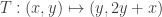$T: (x,y) \mapsto (y, 2y+x)$ in the sector $\{ x < y < 2x\}$ . This time, the determinant is 1, so we are genuinely in $SL(2,{\Bbb Z})$ . The continued fraction algorithm can be viewed projectively as a dynamical system on the first quadrant of the plane which maps $(x,y)$ to $(x,y-x)$ when $y \geq x$ and $(x,y)$ to $(y,x)$ otherwise. This dynamical system terminates for any element of ${\Bbb Z}^2$ by an infinite descent; but when applied to an eigenvector $(x,y)$ of T, it maps to $T^{-1}(x,y)$ after three steps, giving a contradiction again.

The fourth proof has a slight typo: $(p+q)^2$ should be $2(p+q)^2$ . The identity $(p+2q)^2 - 2(p+q)^2 = -(p^2-2q^2)$ is equivalent to the assertion that 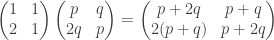$\begin{pmatrix} 1 & 1 \\ 2 & 1 \end{pmatrix} \begin{pmatrix} p & q \\ 2q & p \end{pmatrix} = \begin{pmatrix} p+2q & p+q \\ 2(p+q) & p+2q\end{pmatrix}$ has a determinant which is the negative of the determinant of $\begin{pmatrix} p & q \\ q & p \end{pmatrix}$ . So the sequences $p_n, q_n$ really have to do with powers of the matrix $T := \begin{pmatrix} 1 & 1 \\ 2 & 1 \end{pmatrix}$ , or equivalently the transform $T: (q,p) \mapsto (p+q,p+2q)$ . I think your argument here is basically equivalent to the observation that $T(q,p) \wedge (1,\sqrt{2}) = (1-\sqrt{2}) (q,p) \wedge (1,\sqrt{2})$ , setting up an infinite descent for $(q,p) \wedge (1,\sqrt{2})$ which is incompatible with $\sqrt{2}$ being rational. (Actually, your proof is a little different, it seems to essentially use the fact that $(q,p) \wedge (1,\sqrt{2})$ stays bounded under iteration, while (q,p) goes to infinity, but it is much the same thing.
Terence Tao Says:
October 4, 2007 at 6:32 pm | Reply
Dear Emmanuel,

I think the key to both proofs of Weierstrass’s theorem is that at some point one needs to obtain an approximation to the identity near every point of the domain, since by taking linear combinations of such things one gets a dense subset of C(X). To get the approximation to the identity, it suffices (by closure under multiplication) to get a function which is 1 at a specified point x_0 and less than 1 elsewhere, since one can then raise this function to a large power to improve the quality of the approximation.

It is at this point that proofs (1) and (2) diverge. Proof (2) simply writes down a function with the desired property, e.g. $1 - (x-x_0)^2$ . Proof (1) proceeds by observing that, since polynomials separate points, one can find a function which is 1 at x_0 and less than 1 at some arbitrarily specified other point x_1. One then takes the “min” of several of these functions (exploiting compactness) to get what one needs (modulo controllable errors). There is then an auxiliary step to observe that the min operation can itself be approximated by polynomials, which can be done either by appeal to Weierstrass (which is a little circular, admittedly, unless one then uses proof (2)) or by explicitly writing down an approximant.

So I guess proof (2) is a shortcut version of proof (1), in which one uses the explicit structure of the domain X=[0,1] and of the ring of polynomials to write down polynomial approximations to the identity.
Emmanuel Kowalski Says:
October 4, 2007 at 6:56 pm | Reply
Here’s another example of result where there seem to be quite a few proofs (at least in the sense that books may include two or three): the existence of Brownian motion as a mathematical object.
Here again, I know two apparently different concepts at play:
(1) some kind of abstract existence theorem for stochastic processes, plus a general continuity criterion (Kolmogorov);
(2) writing down an “explicit” (in some sense) sequence of processes which converge (in law) to the required one (Lévy, the invariance principle, Bernstein polynomials, …)

Here I can see a fairly strong link between the two, in that the proof of convergence in law is often (explicitly or not) quite similar to the general continuity criterion. But does it qualify has making the proofs “the same”?
Kenny Says:
October 4, 2007 at 7:14 pm | Reply
In response to John Armstrong, I think the problem with that sort of approach to proof equivalence is that it tends to get bogged down in technicalities very fast, because it focuses too much on the specific syntactic moves in a proof. All sorts of tricky things come up with cut-eliminations (which might apparently change the number of times a rule is invoked in the proof) or even just doing operations in different orders.

This is a very difficult project that people have thought about for a while, but I don’t know if people have really gotten anywhere on it yet. We probably need more good examples, as Gowers is suggesting, to get our intuitions really going, so we can even figure out what criteria a good notion of proof equivalence should satisfy. (Like whether or not it should even be an equivalence relation!)

Or maybe it would help to approach this in some sort of opposite direction? If we start by thinking about what makes “the correct” proof of a theorem, then perhaps that will shed light on what sorts of modifications to a proof are inessential?
John Armstrong Says:
October 4, 2007 at 7:39 pm | Reply
Kenny, you’re right that that specific approach gets bogged down in the specific moves you choose. But, so does the formalist approach to mathematics in general.

We generally “do mathematics” at a much higher level than strict formalism, whether or not we believe in the formalist view. Still, there’s an unspoken analogy between how a high-level mathematical proof works and how a low-level formal deduction works. All I’m saying is that there’s a way of talking about “proof-morphisms” in the formalist approach, and so there should be an analogue of such things in the actual way we do proofs in real mathematics.
Emmanuel Kowalski Says:
October 4, 2007 at 7:42 pm | Reply
Yet another example… (I fiind this very interesting, as people can see…)

There are quite a few proofs of the fact that
$\displaystyle{L(1,\chi)=\sum_{n\geq 1}{\chi(n)n^{-1}}}$
is non-zero for a non-trivial Dirichlet character $\chi$ ; the crucial case is when $\chi$ is a real-valued character (like the Legendre symbol). (And this fact is itself the crucial final ingredient in proving Dirichlet’s theorem on primes in arithmetic progressions)

Here the two most distinct approaches seem in stark contrast: one is the algebraic proof of Dirichlet, which uses the exact class number formula to express $L(1,\chi)$ as an obviously non-zero number (e.g., $L(1,\chi)$ is, in the case $\chi(-1)=-1$ , essentially equal to $h/\sqrt{|d|}$ where $h$ is the class number of an associated imaginary quadratic field), and the other is analytic, and there are many variants, e.g., compare upper/lower estimates for
$\displaystyle{\sum_{n<x}{n^{-1/2}\sum_{ab=n}{\chi(a)}}.}$

Despite the differences, there are very strong links; in particular the inner sum above is the number of ideals of norm $n$ in the quadratic field occuring in the first proof, and this “explains” its properties, in particular that it is $\geq 1$ for $n$ a square (though one does not need the quadratic field to prove this).
However, I wouldn’t say the proofs are “the same”; the first requires as an extra step some form of quadratic reciprocity; moreover, this proof more or less remains stuck there, whereas the other is really the basis for many arguments towards lower bounds for $L(1,\chi)$ , and then for lower bounds for class numbers.
gowers Says:
October 4, 2007 at 11:27 pm | Reply
I’ll see if I can think of some less simple examples, but a fairly elementary situation where two proofs can be regarded as essentially the same is when a proof relies on compactness and you can choose whether to use open covers or convergent subsequences. For example, to prove that every continuous real-valued function on $f$ on $[0,1]$ is bounded we can either assume not and find a sequence $(x_n)$ such that $f(x_n)$ tends to infinity, find a limit point $x$ , and derive an easy contradiction, or we can use continuity to surround each point with an open interval where $f$ is bounded and pick a finite cover of such intervals.

Why do we want to call these two proofs essentially the same? After all, the equivalence between Heine-Borel and Bolzano-Weierstrass, though simple, is not a complete triviality. However,the basic fact one uses in both proofs is the same: that every $x$ is contained in an interval in which $f$ is bounded. The rest of the proof is somehow standard compactness window-dressing: if you want to prove it by contradiction, you use Bolzano-Weierstrass, and if you want to prove it “forwards” then you use Heine-Borel. In general, I think I could justify an assertion along the following lines: if you use Heine-Borel in a proof then you can convert it into a proof using Bolzano-Weierstrass by zeroing in on the fact that you plug into Heine-Borel and plug it into Bolzano-Weierstrass instead.

Of course, this can’t be completely correct, because there are compact topological spaces that fail to be sequentially compact. But I think it’s safe as long as we stick to subsets of $\mathbb{R}^n$ , say.

Just to check, let’s prove that the distance between a closed set $F$ and a disjoint closed bounded set $K$ is positive. The Heine-Borel proof tells us to include each point of $K$ in an open ball that’s disjoint from $F$ . And now I remember something that once worried me, which is that we have to apply a small trick: we cover $K$ by finitely many open balls $B(x_i,\delta_i)$ in such a way that $B(x_i,2\delta_i)$ is disjoint from $F$ . Then if $\delta$ is the minimal $\delta_i$ , we find that the distance from $K$ to $F$ is at least $\delta$ , since each point $x$ is distance at most $\delta_i$ from some $x_i$ and hence distance at least $\delta_i$ from $F$ .

The Bolzano-Weierstrass proof works out more simply. If the result is false, then pick a sequence of points $x_1,x_2,\dots$ in $K$ with $d(x_i,F)$ tending to 0. This has a convergent subsequence, with a limit point $x$ , and we also get a sequence in $F$ that converges to $x$ , so $x\in F$ , by the fact that $F$ is closed, contradicting the disjointness.

The thing that bothered me is that there was no analogue in that proof of the “replace $\delta_i$ by $2\delta_i$ ” trick, whereas usually one likes to feel that it’s impossible to avoid the work in a proof — all you can do is shift it around. It’s doubly strange because in a certain sense compactness is stronger than sequential compactness: it implies sequential compactness more easily than sequential compactness implies it. And yet the proof using sequential compactness was easier.

So perhaps I won’t after all manage to give some precise “translation scheme” for interchanging sequential compactness proofs and compactness proofs.

This reminds me of a very irritating mathematical difficulty I once had and never resolved. A very nice result in Banach spaces was proved (by Nicole Tomczak-Jaegermann) with the help of induction on countable ordinals. All my experience had taught me that such proofs could be converted into equivalent proofs using a double induction. But I was unable to be precise about how, and I never managed to convert that one.
Top Posts « WordPress.com Says:
October 5, 2007 at 2:50 am | Reply
[…] When are two proofs essentially the same? A couple of years ago I spoke at a conference about mathematics that brought together philosophers, psychologists and […] […]
gowers Says:
October 5, 2007 at 9:13 am | Reply
(Just) after a good night’s sleep I think I sorted out my problem in my previous comment. One can prove the theorem about distances between sets by noting that the distance $d(x,F)$ is a continuous function of $x$ , which therefore attains its minimum on $K$ . The latter fact can easily be proved by Heine-Borel. The “key fact” that is then needed is that every point $x$ is contained in a ball, every point of which has positive distance from $F$ . This is what was achieved more constructively with the $2\delta_i$ above. Precisely the same fact is also needed in the sequences proof, but this time it is hidden inside the simple statement that $x\in F$ . How do we prove this? Well, for each $x_i$ in the convergent subsequence we take some $y_i\in F$ such that $d(x_i,y_i)\leq\delta_i$ . We then need to know that the $y_i$ converge to the same limit, and this is the point where addition of distances and the triangle inequality are involved.

So this result does, after all, illustrate the general idea that if two proofs are essentially the same then they should involve the same amount of work. I should, however, qualify that, since it is possible to insert unnecessary work into a proof without changing its essential character. So it might be better to say that they involve the same “irreducible core” of work, or something like that.

A clear message that comes out of Terry’s first comment is that a general way of distinguishing between two proofs is to show that one proof “yields more” than the other. This could be an algorithm, or an efficient algorithm, or an explicit construction, or a generalization (either through a weaker hypothesis or through a stronger conclusion).

Here’s a rather extreme example: the usual combinatorial proof of van der Waerden’s theorem could not be regarded as the same as proving it by first proving Szemeredi’s theorem and then deducing van der Waerden’s theorem, since the latter also gives you a theorem that was an open problem long after the former was first proved. Of course, that counts as putting in unnecessary work if you use one of the proofs of Szemeredi’s theorem that needs van der Waerden’s theorem (or something very similar) as a step along the way. But not all of them do.

This raises another issue, very closely related to sameness of proofs. It’s the idea that one statement can be “stronger” than another. If two theorems A and B are both proved, then in a stupid sense they are equivalent, since each one implies the other. (To prove B just junk A and prove B, and vice versa.) The non-stupid sense in which we use the word “implies” requires a “genuine use” of a statement used to imply another statement. But that’s another fairly hard idea to make precise. (Maybe a category theorist would like to say that A genuinely implies B if there is a proof of B from A that is not homotopic to the proof A implies “0=0” implies B. So now we’re back to sameness of proofs.)

Returning to the word “stronger,” it’s also interesting that we often describe one statement as stronger than another when we are about to prove that the two statements are equivalent. We say that A is stronger than B if “A implies B” is the “trivial direction” of the equivalence. For example, the statement that there is a perfect matching in a bipartite graph is “stronger” than the statement that the graph satisfies Hall’s condition. Or the statement that a group $G$ “belongs to one of these families or else is one of these 26 groups” is stronger than the statement that $G$ is finite and simple.

I mention this just to make the point that, in the light of Terry’s observations, perhaps I should refine my earlier questions. Are there good examples of genuinely different proofs of the same statement that are not different because of their other consequences? If so, then how might one go about showing that they were genuinely different? Here, I’m trying to rule out simple examples such as proving B directly versus proving a much stronger statement A and deducing B. Incidentally, the previous paragraph gives, I think, another way in which two proofs can be different: one proof may use axioms while the other uses a classification theorem and then verifies the statement for each example that comes out of the classification.
James Says:
October 5, 2007 at 10:46 am | Reply
Does anyone know if anyone has created toy logics in which it’s possible to say something interesting about homotopies between proofs?
Emmanuel Kowalski Says:
October 5, 2007 at 4:37 pm | Reply
Coming back to the example of non-vanishing of $L(1,\chi)$ , it comes to me that at a certain (very high) level, the two approaches are “the same”: the algebraic proof and analytic proof can be said to approach the result by deriving it from the fact that the product $\zeta(s)L(s,\chi)$ , where $\zeta(s)$ is the Riemann zeta function, has a pole at $s=1$ . However, the approaches diverge then in how to approach this goal, and I think that at a lower level the difference is genuine.

This suggests that it might be useful to look at similarity of proofs by trying to see at what level — if any — they start to diverge. This makes sense because two proofs of the same statement are identical at the highest level (where the statement itself is seen as an axiom, or a black box for further arguments), so the divergence level is (in a very rough sense) always well-defined.
Danny Calegari Says:
October 5, 2007 at 5:47 pm | Reply
What about the following proof: a rational number is the same thing
as an assignment of an integer to every prime, which is zero for all
but finitely many primes, i.e. a divisor (by uniqueness of prime factorization).
Squaring acts on rational numbers (in this representation) by multiplying all
these integers by 2. So a number is the square of a rational if and only
if all these numbers are even. 2 assigns 0 to every prime except 2, to which
it assigns 1 (which is not even).

This is a “proof by canonical form”: find a canonical form for a certain class
of objects in which the object in question has a form in which the desired
property is obvious. In this respect it’s a little bit like proof 3 above (except
that the canonical form is for 2 rather than for sqrt(2)). Maybe this should
be called the “A=B” method (after Wilf-Zeilberger . .)
gowers Says:
October 5, 2007 at 7:06 pm | Reply
Danny, I like that point. The proof you mention could also be thought of as a proof that uses a classification theorem — in this case classifying the rationals by their multiplicative structure — so it illustrates well what I was trying to say in an earlier comment about another way in which proofs can be different. (But in this case one could perhaps argue that you only need to know how 2 appears in the factorization, and even just the parity, so it’s not quite clear whether one really does want to call it different, or just the same with some extra unneeded stuff thrown in. I’m not sure what my opinion is there.)

While musing on Terry Tao’s remarks about $SL_2(\mathbb{Z})$ I came up with another proof. I was thinking about whether there was a nice infinite set of proofs, of which the first two I gave were just two particularly simple examples. Terry’s suggestion is to think about $2\times 2$ integer matrices with $\begin{pmatrix} \sqrt 2\\ 1 \end{pmatrix}$ as an eigenvector. The general form of such a matrix is $\begin{pmatrix} a&2b\\b&a\\ \end{pmatrix}$ . It was convenient if the determinant was $\pm 1$ , but that gives you the Pell equation $a^2-2b^2=\pm 1$ and means that you’ll end up with powers of the matrix $\begin{pmatrix} 1&2\\1&1 \end{pmatrix}$ already considered. However, here’s a proof based on a matrix with determinant $-2$ .

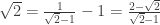
First, observe that $\frac{6-4\sqrt{2}}{3\sqrt{2}-4}$ is equal to $\sqrt{2}$ . Observe also that $6-4\sqrt{2}$ is strictly between $\null 0$ and $1$ . It follows that if $p/q$ is a fraction that equals $\sqrt{2}$ , then $\frac{6q-4p}{3p-4q}$ is a smaller fraction that also equals $\sqrt{2}$ . I haven’t yet worked out the most general proof along these lines.

A rather silly argument that combines the first two proofs I gave earlier is to use a matrix with an entry that is half an odd integer. It’s possible to use a suitable matrix of this kind to convert $p/q$ into a smaller fraction, but you need the fact that $q$ is even to be sure that that the numerator and denominator of the smaller fraction are integers. I won’t embarrass myself by putting up the details.
gowers Says:
October 5, 2007 at 9:51 pm | Reply
A thought that occurred to me a while after reading Emmanuel’s last comment, and also connected with the different proofs of the irrationality of $\sqrt{2}$ , and indeed Terry’s idea of thinking about constructions, is this. Often a mathematical statement begins with a universal quantifier, but to prove it one ends up needing to construct something. To take an example, we might decide to prove the irrationality of $\sqrt{2}$ by infinite descent, and then decide that what we needed was a $2\times 2$ integer matrix with $\begin{pmatrix}\sqrt{2}\\ 1\\ \end{pmatrix}$ as an eigenvector with eigenvalue less than 1. This approach to the problem then turns into the problem of constructing such a matrix, which can be done in many different ways. Given two such constructions, one might say that the proof was the same at the top level (since the idea for proving the universally quantified statement was the same) but different at a lower level (since the idea for constructing a matrix was different).

Actually, in this example you don’t really need much of an idea to find the matrix. You just note that it has the form $\begin{pmatrix} a&2b\\ b&a\\ \end{pmatrix}$ and find that all you need to make the proof work is to satisfy the inequality $0<a+b\sqrt{2}<1$ . Above, I took $a=-4$ and $b=3$ , but obviously one can find many many other examples: indeed, for any non-zero integer $b$ there is an $a$ that does the job (though, amusingly, I’m using the irrationality of $\sqrt{2}$ when I say that).
manuel Says:
October 7, 2007 at 11:37 pm | Reply
Can we prove that there is no bijection between the integers and the real numbers without using a “diagonal argument”? Could this be a result with essentially one proof?
Jonah Sinick Says:
October 8, 2007 at 8:44 am | Reply
Manuel,

Cantor’s original proof that the real numbers are uncountable is (essentially) as follows:

We claim that no sequence f(n): N —> [a, b] is onto. Let f(n) be any sequence and let a_1 < b_1 be the first two distinct members of the sequence f(n). Then f(n) must attain at least two distinct values in [a_1, b_1], call the first ones a_2 < b_2.

By completeness of the reals the above sequence of nested closed intervals has a nonempty intersection. Say c is in the intersection. If f(N) = c then since c is in [a_N, b_N] we have N > 2N which is impossible. So c must not be in the image of f(n).

Should this proof be regarded as essentially the same as the diagonal argument? I’m not sure. My own judgment is that it is because at bottom both proofs are applications of the completeness of the reals (as they must be!) and don’t depend on any other properties of the reals. But this judgment seems highly subjective to me.

How about the usual approaches to the fundamental theorem of algebra?
http://en.wikipedia.org/wiki/Fundamental_theorem_of_algebra#Proofs
I consider the proofs listed in the wikipedia article under complex analysis and topology to be “essentially the same” as one another while the proofs listed under “algebraic proofs” seem essentially different from the proofs by complex analysis and topology. I would be interested in others’ responses to this example.
Jonah Sinick Says:
October 8, 2007 at 8:47 am | Reply
… f(n) must attain at least two distinct values in [a_1, b_1], call the first ones a_2 2i….

I’m genuinely perplexed at why my comment typeset so poorly. I apologize for the boldface letters.
gowers Says:
October 8, 2007 at 10:43 am | Reply
Jonah, I’ve corrected your first comment so that it looks OK — you’d put < instead of “ampersand lt semicolon” and because the next letter was a b you ended up with a lot of bold face. In general, I’ve got a policy of quietly editing people’s comments when they don’t compile properly. I don’t change what anyone says though.

I’ve thought about the two proofs of the uncountability of the reals, and in my view they really are the same. Here’s a slight variant of Cantor’s argument as presented by you. Suppose that $[0,1]$ is countable, and enumerate it as $a_1,a_2,\dots$ . Then inductively construct nested closed intervals $\null [ p_{n}, q_{n} ]$ of positive length such that $a_n\notin [p_n,q_n]$ . This is obviously possible, and can be done in many different ways. (Your argument is different only in that you chose a specific way of constructing these intervals, which happened to depend on the sequence $(a_n)$ .) Then an element of the intersection of the intervals $\null [p_n,q_n]$ cannot be any of the $a_n$ .

To turn that into the usual diagonal argument, you simply choose $\null [p_n,q_n]$ to be an interval of all points with a given first $n$ digits in their decimal expansion (except that it’s slightly more convenient to take the right end-point of this interval as well). You choose the $(n+1)$ st digit to be 3 or 6 according to whether the $(n+1)$ st digit of $a_n$ is or is not one of 5 or 6, say.

So this fits nicely into the scheme of what I was mentioning earlier. We actually prove a more precise statement: for every countable sequence $(a_n)$ of reals (in $[0,1]$ ) there is a sequence of nested closed intervals $\null [p_n,q_n]$ such that $a_n$ does not belong to $\null [p_n,q_n]$ . In some sense, the proof of the “for every” part always seems to be the same, while the proof of the inner “there is” part can be done in many different ways. But demonstrating the “there is” part is sufficiently simple that these different approaches don’t really feel all that different. Or perhaps the real reason is that one can describe a sort of “nondeterminate algorithm” (with steps like, “If $a_n$ is less than $q_n$ then pick $p_{n+1}$ and $q_{n+1}$ such t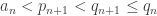hat $a_n<p_{n+1}<q_{n+1}\leq q_n$ “) and the “different approaches” that we want to identify consist in making this algorithm determinate — or, if you prefer, in different proofs that the indeterminate steps can be specified precisely.

Going back to the original question of Manuel, I think it would be very interesting to show that any proof, or perhaps any “sensible” proof, of the uncountability of the reals must involve a diagonal argument of some sort. It certainly seems to be the case. Recasting it in the terms of the last paragraph makes it almost obvious that it is the case, but I haven’t quite demonstrated that you have to use the nested closed intervals property. However, one does have the basic problem, “Given a sequence $(a_n)$ , construct a real that is not an element of the sequence.” Since the reals are defined as limits of sequences in one way or another, one does seem to be forced to construct another sequence in such a way that its limit is not one of the $a_n$ . And then one appears to be forced to deal with each $a_n$ in turn, and the obvious way of constructing a sequence that does not have $a_n$ as a limit is to make sure that eventually it lives inside a closed interval that does not contain $a_n$ . Actually, that’s equivalent of course. One could do stupid things like not ensuring that the sequence avoids $a_n$ until you reach the $2^n$ th term of the sequence. This would be like taking not the obvious diagonal but something similar that did the job equally well. I’d say that this paragraph is a fairly convincing informal argument that there is essentially only one proof of the uncountability of the reals, but I’m not sure how I’d go about making it more formal.
gowers Says:
October 8, 2007 at 11:02 am | Reply
One more thought. Here’s a proof of uncountability of the reals that probably ends up being the same, but it might take a bit of thought to see how. You first prove that there is a countably additive measure on the reals that gives the usual length to open and closed intervals. Then the measure of a countable set is zero while the measure of $[0,1]$ is 1.

A good place to start if one wants to see why this is the same proof is the exercise (the significance of which I understand after reading Imre Leader’s forthcoming article on measures for the Princeton Companion) of showing that if $I_n$ is an interval of length $a_n$ and if the $a_n$ s sum to less than 1, then the intervals $I_n$ cannot cover all of $[0,1]$ . You need this to get going with measure theory and it depends fundamentally on the completeness of the reals.
gowers Says:
October 8, 2007 at 2:28 pm | Reply
Actually, here’s a more detailed answer to whether the “measure-theoretic proof” is just the usual proof in disguise. The Lebesgue measure of a set X is the infimum of the sum of lengths of a countable collection of intervals that covers X. It’s easy to prove that the measure of a countable set is zero, but how do you prove that the measure of the interval $[0,1]$ is not zero? You take any countable collection of open intervals with lengths adding up to less than 1/2, say, and prove that the union of this collection is not the whole of $[0,1]$ . The reason it isn’t is that if $U_n$ is the union of the first $n$ open intervals, then the complement $F_n$ of $U_n$ is a finite union of closed intervals of total length at least 1/2. (This is because if you write $[0,1]$ as a finite union of intervals, whether open or closed, then their lengths must add up to at least 1, a fact that is easy to prove.) Therefore, the sets $F_n$ are a nested collection of non-empty closed sets, so they have a non-empty intersection.

This appears to be a slightly more general argument, as it involves nested intersections of closed sets that are more general than intervals. Moreover, that is necessary: if you try to find your point that is not in the union of the open intervals by constructing an intersection of closed intervals, you can’t keep the $n$ th closed interval large enough to guard against one of the later open intervals containing it. And perhaps the reason we have a somewhat different proof is that we have proved something stronger: instead of merely showing that a countable union of intervals of length 0 cannot be all of $[0,1]$ we’ve shown it for a countable union of intervals of any lengths that add up to less than 1 (if we’re prepared to modify the argument a tiny bit).

But even this doesn’t make it a genuinely different proof of the uncountability of the reals , any more than it would be a genuinely different proof if we first used the diagonal argument and then said, “Oh, and by the way, here’s a proof of Fermat’s last theorem thrown in.” If we just want to prove that the set $\{a_1,a_2,\dots\}$ isn’t all of $[0,1]$ then we can choose any old open intervals around the $a_i$ and use the measure-theoretic argument to prove that their union is not all of $[0,1]$ . But if we’re allowed to do that, then we can make their sizes go to zero sufficiently rapidly that it is possible to use nested intervals for the argument, rather than more general nested closed sets.

Despite all that, maybe one could say that there is in fact a very slight difference between the two approaches. If you prove the result using nested intervals, then there is a tiny effort needed to construct those intervals. If you use more general closed sets, then you can simply take the complement of the open sets you are considering, so constructing the closed sets no longer takes any effort, but now you are looking at more complicated sets.

The proof that a nested intersection of non-empty closed subsets of $[0,1]$ is non-empty is basically the same as the proof for intervals: their infs tend to a limit that belongs to the intersection. However, maybe this shouldn’t quite make us think that the proofs are essentially the same because if you generalize to higher dimensions it does seem to be genuinely harder to prove that a nested intersection of arbitrary closed sets (or even of finite unions of closed boxes) is non-empty than it is if those sets are just boxes: the inf trick no longer works.
Scott Carnahan Says:
October 8, 2007 at 6:47 pm | Reply
The Kazhdan-Lusztig conjecture was proved by translating the question through several areas of mathematics, until it reached a form that could be treated by Deligne’s theory of weights. At the end of Bernstein’s D-module notes, he mentions that one wouldn’t need to go through the business of varieties over finite fields if one had a satisfactory theory of mixed Hodge modules (does this exist now? I’m behind on recent developments). Let’s suppose such a theory existed, and we had a proof using it. Would such a proof be equivalent? If we had a good theory of mixed motives, I suppose one could claim that both proofs were equivalent, since we would be using two realizations of the same machine. At least, I imagine this is what Bernstein had in mind. My question is, are two proofs equivalent if the equivalence requires a conjecture?
Scott Carnahan Says:
October 8, 2007 at 7:08 pm | Reply
Here’s another example: three proofs of the Weil conjectures. I think Deligne’s original proof used a lot of l-adic monodromy on Lefschetz pencils, Laumon’s proof used some kind of sheafy Fourier transform, but still revolved around the l-adic cohomology theory set out in SGA, and Kedlaya’s proof also used a sheafy Fourier transform, but in the language of p-adic differential equations. Kedlaya said that he was guided by strong analogies between the l-adic and p-adic worlds, but formalizing this as an equivalence of proofs seems a bit ambitious with our current state of knowledge.
gowers Says:
October 9, 2007 at 12:48 am | Reply
My gut feeling (but no more than that) about whether two proofs can be equivalent if the equivalence is just a conjecture is that they can. It seems to me to be a bit like the two-dimensional equivalent of asking whether a mathematical statement can be provable if it is just a conjecture. Also, it seems clear that two proofs can be equivalent in a highly non-trivial way, so why not in a way that is so non-trivial that it actually depends on an unsolved conjecture? However, coming up with good examples of such a phenomenon is very interesting.

On a more mundane note, a fairly simple example of a result that seems to have genuinely different proofs is Fermat’s little theorem. I know of three: the deduction from Lagrange’s theorem, the deduction from the fact that multiplying by $a$ permutes the non-zero elements of $\mathbb{F}_p$ and the inductive proof based on the fact that the binomial coefficients $\begin{pmatrix} p\\ k\\ \end{pmatrix}$ are multiples of $p$ when $1\leq p<k$ . Can anyone identify any two of those proofs? (It might be possible for the first two, perhaps.)

Another question for algebraic number theorists out there. Gauss’s law of quadratic reciprocity famously has a vast number of proofs. How many genuinely distinct proofs are there? Even a rough estimate would interest me.
Emmanuel Kowalski Says:
October 9, 2007 at 6:29 am | Reply
Coincidentally, I was just reading yesterday one of Euler’s proof of Fermat’s little theorem in a translation of his original paper. It’s essentially the first one mentioned above, tailored to the case of a cyclic group (and with unusual style and notation as one would expect) but clearly recognizable. What’s interesting is that at the end Euler specifically states that this is a completely different proof from the one with binomial coefficients, because it leads to many other results. (Those are essentially his words, though I don’t have the book handy just now to quote it).

Concerning quadratic reciprocity, this
site of F. Lemmermeyer lists 224 published ones, and classifies them roughly (and has references), which seems to indicate that the number of fairly distinct ones is maybe 40 or 50. I think one can identify some of these (e.g., many arguments are based on Gauss sums or cyclotomic fields, and these can be certainly made to correspond in some cases), but that would probably leave at least 10 genuinely different arguments.
James Cranch Says:
October 9, 2007 at 11:07 am | Reply
I guess a lot of things traditionally called “metatheorems” supply examples of transformation techniques for proofs.

Category theory has several. There’s the “duality principle”: that the axioms of category theory are unchanged by reversing the directions of all the morphisms and all the compositions, and so every time you prove something about the situation one way around, you can rewrite the proof to prove a dual statement.

I suppose that, logically, that’s a different thing: the rewriting process here yields a proof of a different statement. But there’s no reason not to be interested in such things.

For an honest example, there’s Freyd’s embedding theorem. The textbook statement is that any abelian category can be embedded fully and faithfully into a category of modules. But the point, philosophically, is that it allows you to prove things in abelian categories by imagining you’re working in a category of modules. In particular, you can “choose elements” of your objects, even though they’re just objects of an abstract category, and don’t really have elements. There is a rewriting technique which replaces such a proof using “elements” with one that doesn’t abuse notation in this manner.
Gil Kalai Says:
October 9, 2007 at 7:14 pm | Reply
This is a very interesting post! I noticed that assertively claiming that two very different proofs of the same theorem are essentially equal is something which can gain you a lot of respect. It shows not only a complete understanding of the two different proofs but understanding deep connections that nobody else see. Maybe one can gain even more respect by claiming that two different proofs for two entirely different theorems are essentially the same but here some caution is advised.

Concerning the question of when two proofs are equal or similar or different, one formal aspect regarding proofs of existence (like fixed point theorems) is the complexity classes of Christos Papadimitriou. These classes can be regarded as a rough (computational complexity) classification of mathematics’ basic tricks and this may lead to a formal notion of different proofs. (In this classification 2 proofs leading to polynomial algorithms are equivalent.)

Here are a few test cases for equality and inequality of proofs:

1) I have a friend who always tell me that the inductive proof of the crossing number inequality (recently featured in Terry’s blog) given by Ajtai Chvatal Newborn and Szemeredi is equivalent to the probabilistic proof. This always surprised me since to me they look different (and in particular I feel that I understand much better the probabilistic one.)

2) There are many proofs of Cayley formula for the number of trees on n labeled vertices. (A book of J W Moon lists quite a few and there are many more.) Can you classify them?

3) Turan’s theorem for the number of edges for a graph on n vertices required to guarantee a triangle has many proofs, and it almost looks that any strategy to prove is doomed to succeed. Which of these proofs are different?
Gil Kalai Says:
October 10, 2007 at 1:06 am | Reply
Regarding the related question when two proofs are entirely different, there are some cases where there is a clear difference between two types of proofs e.g. the distinction between constructive/non constructive proofs; effective/non-effective proofs; Proofs based on randomized construction/ proof based on explicit construction. In these three cases one type of proofs is usually much harder than the other.

This reminds me also of the long-time mathematical endeavor of finding an “elementary proof” of the prime number theorem. The precise meaning of “elementary proof” in this case was not entirely clear to me. (At some points I convinced myself that the distinction is manifested in that the “elementary proofs” apply to certain formulations of the PNT when you replace all primes by a dense subset of primes; but I am not sure this is correct.)

In all the cases above entirely different proofs reflect a different mathematical task to start with. It can be interesting to bring more examples of entirely different proofs for (really) the same theorem, when the distinction is not of the nature that one proof (to start with) tries to achieve some much harder goal (effective; constructive; explicit; elementary; bijective, not using CH; computerized; not computerized; etc..)
Gil Kalai Says:
October 10, 2007 at 5:03 am | Reply
I forgot another case of distinction between proofs which is the case of simple proofs vs difficult proofs. Unlike the distinction between effective/non-effective; constructive/non constructive, etc., there is something paradoxical about the (all important) endeavor of finding simple proofs for difficult theorems. To start with, there is a strong positive correlation between the difficulty of the proof and the difficulty of finding it. But finding simple proofs for difficult theorems is usually very difficult.

It is like the well known paradox:

Rare things tend to be more expensive;

Cheap horses are rare;

Therefore, cheap horses tend to be more expensive.

(Finding difficult proofs for easy theorems is also quite interesting from time to time.)
Ryan Reich Says:
October 10, 2007 at 5:49 am | Reply
One rather famous distinction between types of proof is in algebraic geometry: the proof via “complex analytic methods” versus the proof via “algebraic methods”. The former includes using just about any facet of the ordinary topology on a complex variety, so for example, one has Poincare duality proven either as Poincare might have, or the way Artin did. Of course, Artin proved it for etale cohomology, but he also proved a comparison theorem that relates that to singular cohomology, so it seems there are two proofs which cannot, even in principle, be reduced to the same thing (since the etale cohomology theorem applies to varieties in positive characteristic too!). I am no doubt revealing my ignorance by trying to talk about this, however…

Actually, it seems to me that anything that can be proven with complex analysis or with something else will have two essentially different proofs; complex analysis is good like that. There is, for example, an amusing computation of the Fresnel integral $\int_0^\infty \frac{\sin x}{x} dx$ using differentiation under the integral sign: let $I(t) = \int_0^\infty e^{-tx} \frac{\sin x}{x} dx$ , observe that the derivative can be computed by elementary means, and that I(t) vanishes as t approaches infinity. That gives you a differential equation which you can solve and then plug in t = 0. You can also do it using the residue theorem, which involves integrating over a triangular contour; I have trouble seeing how these could be the same proof. Perhaps they are, though.
Emmanuel Kowalski Says:
October 10, 2007 at 8:15 am | Reply
In the case of the Prime Number Theorem, the stated goal (e.g., in one of Hardy’s lectures on Ramanujan’s work, if I remember right) was to find a proof that does not use complex analysis. It was hoped that this would imply significant new insight into the study of prime numbers, especially with respect to those problems that were then still unsolved, such as the Goldbach, prime $k$-tuples, conjectures. However, the proof of Selberg (and Erdös) didn’t really have such an effect, and elementary proofs have not yet recovered the same results provided by the standard complex-analytic proofs (with respect to remainder terms, and uniformity in arithmetic progressions).
im Says:
October 10, 2007 at 5:51 pm | Reply
With all this discussion of elementary vs non-elementary proofs, is there scope for a loop back to your wonderful earlier post on Cauchy’s theorem as generalization of f’=0 => f = constant?
Scott Carnahan Says:
October 10, 2007 at 10:58 pm | Reply
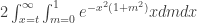
I’ve seen two proofs that $\int_0^\infty e^{-x^2} dx = \frac{\sqrt{\pi}}{2}$ . The first one is the standard proof using Fubini and polar coordinates. The second involves constructing two functions 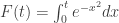$F(t) = \int_0^t e^{-x^2} dx$ and $G(t) = \int_0^1 \frac{e^{-t^2(1+x^2)}}{1+x^2} dx$ , and noting with derivatives that $(F(t))^2 + G(t)$ is constant. It seems quite beautiful, and I learned it from W. Luxemburg.

I’m curious if there is an analytic reason for someone to come up with the function G, because it seems to come out of nowhere. It might also suggest some way that these two proofs are equivalent.
gowers Says:
October 11, 2007 at 11:47 am | Reply
Scott, that’s an interesting challenge. It looks to me as though there might be a perspective from which those two proofs could be similar in a way that has been discussed in earlier comments: that they have the same basic strategy, but that that strategy involves constructing something that can be constructed in many different ways. However, in this case the construction is a sufficiently non-trivial process for it to be questionable whether one would want to regard the proofs as the same. I haven’t worked this out properly but let me say why I think it looks like a possibility.

The quantity $(F(t))^2$ can be regarded as the integral of $e^{-x^2-y^2}$ over the square $\null [0,t]^2$ . Thus, one could regard $(\sqrt\pi/2)-G(t)$ as a guess for what that integral ought to be (but at the moment I don’t see how the guess was made) and the differentiation trick as just a verification that the guess is correct. The first proof could be regarded as using the formula 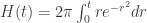$H(t)=2\pi\int_0^t re^{-r^2}dr$ as a guess for what the integral of $e^{-x^2-y^2}$ ought to be over a circle of radius $t$ . Probably that can be proved correct by differentiation as well.

Thus, it looks to me as though the basic strategy is, “Find a two-dimensional set on which you can work out the integral of $e^{-x^2-y^2}$ .” (Of course, I really mean a set that grows with a parameter $t$ .) Once you’ve had that idea, it turns out that there is more than one such set.

Having said that, the formula for $G(t)$ does seem rather non-obvious and seems to involve a distinctly “new idea.” Most notably, unlike in the circle case, it gives an integral that (as far as I can see) is just as hard to calculate as the original one, but which happens to behave very nicely when $t$ is 0 or infinity. So it would be very interesting to know where this comes from, and also whether there are any other proofs that fit into this general scheme.
gowers Says:
October 11, 2007 at 2:09 pm | Reply
On second thoughts, perhaps it doesn’t take an idea to come up with $G(t)$ so much as a leap of faith that the integral over the square will be easy to calculate, coupled with the thought (which is fairly standard, so perhaps not quite an idea in the true sense) that it might be worth differentiating it to see what one gets. If you do, then you want to calculate $2F(t)F'(t)$ , which works out to be $2\int_0^t e^{-t^2-x^2}dx$ . It’s quite natural to make the substitution $x=ty$ , which leads to $\int_0^1 2te^{-t^2(1+y^2)}dy$ . Then it’s quite natural to notice that the integrand can be antidifferentiated with respect to $t$ , so this is 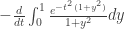$-\frac{d}{dt}\int_0^1\frac{e^{-t^2(1+y^2)}}{1+y^2}dy$ . And now we obviously want to use the fundamental theorem of calculus, so we want to evaluate this integral for $t=0$ and $t=\infty$ … and we can.

The initial leap of faith isn’t really a piece of magic, since the square and the circle are the two simplest two-dimensional sets that one might try. So the above seems to me to be a plausible account of how the function $G$ might have been discovered.
David Speyer Says:
October 11, 2007 at 2:11 pm | Reply
I think I see why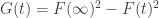 $G(t)=F(\infty)^2-F(t)^2$ . The right hand side is the integral of $e^{-x^2-y^2}$ over the complement of the square $\null [0,t]^2$ . By the symmetry of the problem over the line $x=y$ , this is
$2 \int_{t \leq y \leq x} e^{-x^2-y^2} dx dy$ .
Now, make the substitution $y=mx$ to get
$2 \int_{x=t}^{\infty} \int_{m=0}^1 e^{-x^2 (1+m^2)} x dm dx$ . The integral on x is now elementary (substitute $u=x^2$ ) and I think the remaining integral on m is your formula for $G(t)$ .

This can be seen as similar to, but not quite the same as, the standard proof. In the standard proof, we change to polar coordinates $\null (x,y)=(r \sin \theta, r \cos \theta)$ . Then the integral on r is elementary and the integral on $\theta$ is trivial. In the new proof, we change to “(slope, intercept)-coordinates”: $(x,y)=(x,mx)$ . The integral on x becomes elementary for the same reason that the integral on r did previously.

This suggests to me a general strategy of proof. Choose any parametrized convex curve $(f(u), g(u))$ cutting off a corner of the positive orthant. Make the substitution $(x,y)=(r f(u), r g(u))$ . The integral on r will always be elementary; hope that you can deal with the integral on u. So the standard proof is to cut off the corner with a quarter-circle, and the modified proof is to cut it off with a square.
David Speyer Says:
October 11, 2007 at 2:14 pm | Reply
Gaah! I can’t get my TeX back to see what went wrong! The first formula that didn’t parse should be $\null [0,t]^2$ — I was just making sure we all knew what I meant by “the square”. The second formula that didn’t parse was just the expression for polar coordinates $(x,y)=(r \cos \theta, r \sin \theta)$ .
gowers Says:
October 11, 2007 at 2:20 pm | Reply
David, I’ve noticed that for some strange reason WordPress doesn’t seem to recognise closed intervals if they occur at the beginning of a LaTeX expression, even if you’ve done everything completely correctly. But I’ve discovered a stupid trick that deals with the problem: instead of writing “latex [0,1]” inside the dollars I write “latex \null [0,1]”. Ridiculously, that seems to cure it. I’ve edited your two comments above so that they do parse, partly using that trick and partly removing a backslash that had attached itself to the letter r in “r \sin \theta”.
Scott Carnahan Says:
October 12, 2007 at 12:17 am | Reply
This seems to be a pretty satisfying answer. David’s general strategy also works well if you decompose of the lower half of the quadrant into hyperbolas and do a hyperbolic trig substitution. However, the square version seems to be special in that it produces a one-dimensional proof in a way that the other two do not, in the sense that a first-term calculus student could parse it without knowning Fubini.

I’ve encountered a similar vanishing problem in LaTeX itself, when I tried to start some aligned equations with a Lie bracket, so it might not be a problem with WordPress. By the way, you can find the original TeX in the alt text of the image.
gowers Says:
October 12, 2007 at 10:54 am | Reply
Here are two proofs that a dense subset of $\{1,2,\dots,N\}$ must contain a “Hilbert cube” of dimension $k$ : that is, a subset of the form $\{x+\epsilon_ia_i:\epsilon\in\{0,1\}^k\}$ . More precisely, for any $\delta>0$ there exists an $N$ such that any subset $A$ of $\{1,2,\dots,N\}$ of size at least $\delta N$ must contain such a set (with the $a_i$ not equal to zero). I’ll just sketch the arguments very briefly.

The first approach is to find (using an averaging argument) some $a_1$ such that the intersection of $A$ with $A-a_1$ is reasonably large. (It’s not too hard to get $\delta^2$ times an absolute constant.) Then you are left needing to find a $(k-1)$ -dimensional cube in this intersection, which you do by induction.

The second approach is to prove a stronger result, namely that you can find $a_1,\dots,a_k$ such that for a significant proportion of $x$ the cube defined above is a subset of $A$ . This you can prove as follows. By induction the result is true for $k-1$ . This gives you $a_1,\dots,a_{k-1}$ and a big set $B$ of $x$ such that the corresponding cube is a subset of $A$ . Since $B$ is dense, some difference occurs frequently in $B$ , and you can make this difference your $a_k$ .

This illustrates a phenomenon that occurs frequently. You want to prove a statement $\forall k P(k)$ by induction. You can either use a simple argument to deduce $P(k)$ from $P(k-1)$ or you can use $P(k-1)$ to deduce $P(k)$ from $P(1)$ (which itself is proved by a simple argument). In other words, you can think of $k$ either as $1+(k-1)$ or as $(k-1)+1$ .

Often the work needed is more or less the same, as the above example illustrates. But sometimes one approach seems to be rather easier than the other (unfortunately I haven’t managed to think of any examples yet), and I’m not sure that I believe in a general principle that says that one can always convert one sort of inductive proof into the other. So perhaps we have here a grey area, where proofs can be similar but it’s not obvious whether we should regard them as the same.
davidspeyer Says:
October 12, 2007 at 3:43 pm | Reply
Oh! I know that LaTeX bug. It occurs when your TeX code is being fed as a parameter into a macro somewhere, and LaTeX, failing to “quote” the square bracket, interprets it as an additional optional parameter to the macro. The most common way I know to produce this bug is to have an item in a list that starts with a square bracket (arguably, this case is a feature.) For example, this LaTeX should cause trouble:

There are two types of parenthesis used in some-programming-language-or-other:
\begin{enumerate}
\item (), used to control the order of operations
\item [], used to call a function or index into an array
\end{enumerate}

The standard solution is to write {[}.
davidspeyer Says:
October 12, 2007 at 4:16 pm | Reply
Here is an example, in elementary number theory, of the phenomenon Prof. Gowers discusses in his previous post. We write ${[}a_1,...,a_n]$ for the continued fraction $a_1+1/(a_2+1/(a_3+...+1/a_n)...))$ . Define $P_n(a_1, ..., a_n)$ by the reucrrence
$P_n(a_1, ..., a_n)=a_n P_{n-1} (a_1, ..., a_{n-1})+P_{n-2}(a_1, ... a_{n-2})$
with initial conditions $P_{-1}=1$ , $P_{0}=0$ . Define $Q_n$ by the same recurrence with $Q_{-1}=0$ and $Q_{0}=1$ . Then a basic result about continued fractions is
${[}a_1, ..., a_n]=P_n(a_1, ..., a_n)/Q_n(a_1,...,a_n).$

Every student that I have ever seen try to prove this (I taught at PROMYS for four years) tries to use induction, starting from
${[}a_1,...,a_n]=a_1+1/[a_2,...,a_n]$ .
This proof can be made to work, but it is hard. However, there is a very easy proof if you start from
${[}a_1,...,a_{n-1}, a_n]=[a_1,...,a_{n-1}+1/a_n]$ .
I think there is a mental block against doing it this way, because the terms in the continued fraction will no longer be integers, but it produces a much simpler proof.
Adam Chmaj Says:
October 19, 2007 at 7:54 am | Reply
To me, the first proof is analytical, the other three algebraic.
Besides, good problems have unique solutions.
- observer Says:
  January 22, 2011 at 12:37 pm
  Number theoretic uses Bezout: Let w=sqrt2=a/b. (a,b)=1 so there are integers c,d, such that ad-bc=1.
  0=(a-bw)(c+dw)=ac+adw-bcw-bdw^2=ac-2bd+w,
  thus w is an integer.
gowers Says:
October 23, 2007 at 10:39 am | Reply
Here’s another example of a result with two proofs that look different and are both quite simple. Perhaps they can be unified — I have not tried.

The statement to be proved is that every finite subgroup of the multiplicative group of non-zero complex numbers must be the group of all $n$ th roots of unity, for some $n$ . This question came up on a Cambridge question sheet for a first-year course on groups, and this term I am what we call a “supervisor” for the course (that is, I see students in pairs and discuss their solutions and attempted solutions).

Here’s the proof that occurred to me. Let $G$ be such a group. Then any element of $G$ has finite order (something that had been proved in an earlier question via the usual pigeonhole-principle argument), and therefore must be a root of unity. Now choose an element of $G$ with minimal argument. If that doesn’t generate the whole of $G$ then a Euclid-algorithm style calculation shows that its argument isn’t minimal — contradiction.

This was the very first question sheet of the course, so I think that was the intended proof, but one of my students suggested using Lagrange’s theorem instead. That quickly leads to a short solution: every element of $G$ must be a $|G|$ th root of unity, and there are only $|G|$ of them, so we are done.

These two proofs certainly have quite significant surface differences: the second uses a piece of algebra that can’t immediately be read out of the first, and the first uses the minimal argument, which doesn’t seem to come into the second. So any unification would have to be from a deepish perspective. Or perhaps they really are different proofs.
E.Bz. Says:
October 23, 2007 at 11:42 pm | Reply
I think you can get enough of Lagrange from the first argument in this situation. Your Euclidean algorithm/ minimal argument is basically exactly how one proves that subgroups of cyclic groups are cyclic – it is then pretty easy to prove that you have Lagrange for the cyclic groups so I suppose there is some similarity. Beyond that I guess they are intrinsically different.
Simon Morris Says:
October 24, 2007 at 10:16 am | Reply
The second proof generalises to (for example) the quaternions, but I can’t see how the first proof would. More convincingly (to me), the first proof also shows that the group is cyclic, whereas the second proof doesn’t. I don’t think I’m missing some small variation of the second proof that would show this, because the transliteration of the second proof to the quaternions certainly couldn’t.

But I’m not sure which subset, if any, of those observations really shows that the proofs are different.
gowers Says:
October 25, 2007 at 6:29 pm | Reply
Simon, I don’t think I understand what you are saying about quaternions. For instance, $G$ could be the group $\null \{\pm 1, \pm i, \pm j, \pm k\}$ , which is not cyclic. The second proof would break down because there are more than eight 8th roots of unity, and the first hardly gets started. But perhaps you had a different generalization in mind.

I also don’t quite understand what it means to say that the second proof doesn’t show that the group is cyclic: if it shows that it’s the group of $n$ th roots of unity then surely it does.
Simon Morris Says:
October 25, 2007 at 7:43 pm | Reply
Sorry – the “generalization” I had imprecisely in mind was just that $G$ consists of $n$ th roots of unity, not that it is all of them, which isn’t a generalization of the result you gave.

I think the first proof shows in passing, as part of its argument, that the group is cyclic, whereas with the second proof, you have to go back at the end and look at the group you’ve proved you have, and check that it’s cyclic. I’m not sure whether that’s a real distinction between the proofs. My rather poor point about the quaternions was just that $G$ needn’t be cyclic there, so there can’t be any generalization of the first proof there that uses some other definition of minimal element. Now that I’ve looked at some of your web pages, I see that I was thinking vaguely along the lines of “quaternions are another model for the complex numbers”, in a way slightly reminiscent of your page about why it isn’t obvious that the integers are bounded in the reals.
Maurizio Says:
November 29, 2007 at 5:07 am | Reply
I’m surprised by the amount of insight about algebraic number theory that i gained reading your proof of the irrationality of $\sqrt{2}$ , i mean it really helped me to better understand many things that i was supposed to already know.

Actually the first two proofs are quite similar if you think about valuations: a valuation is a multiplicative function from a field to $\mathbb{R}^+$ that respects the triagular inequality, ie $v(ab)=v(a)v(b)$ and $v(a+b) \leq v(a)+v(b)$ , and $v(a)=0$ only if $a=0$ . It can be proved that all such valuations over the rational number are (up to equivalence) the usual absolute value ( $v_\infty(a)=|a|$ ) and given by prime numbers ( $v_p(p^k\frac{a}{b})=\frac{1}{p^k}$ , where $a$ and $b$ are prime with $p$ ), so they can be thought of as a suitable generaliation of prime numers and ideals, providing additionally a “prime at infinity”. All valuations share important properties, for instance they induce a topology with respect to which you can take the completion, etc.

In the first proof of the irrationality of $\sqrt{2}$ , you are taking a fraction $\frac{p}{q}$ where $p$ and $q$ minimize the valuation at the prime 2 (by dividing the numerator and denominator by the biggest common power of 2), and you get an absurd because $v_2(\frac{p^2}{q^2})$ cannot possibly be equal to $v_2(2)$ . In the second proof, you are choosing $p$ and $q$ with smallest absolute value (and so smallest valuation at $\infty$ ), and then apply a tranformation (an element of $SL_2(\mathbb{Z})$ ) that leaves the value of the fraction, supposed to be equal to $\sqrt{2}$ , unchanged, but decreases the valuation at $\infty$ of the denominator, absurd by minimality. So, by what i’m understanding, most of the difference in the proofs comes by how the “non-archimedean” valuation at 2 and the “archimedean” one at $\infty$ work, possibly an experienced number theorist may give us a better explaination of this fact.
uri Says:
December 17, 2007 at 12:26 am | Reply
Hi,

Can’t leave it unsaid that the second proof mentioned for the irrationality of $\sqrt{2}$ can be seen in a beautiful manner:

Take an actual triangular piece of paper of sizes p,p,q (assuming $p^2=2q^2$). You can now fold one of the sides on the diagonal, and get yourself a smaller triangle of sizes $p-q,p-q,2q-p$, revealing that $2(p-q)^2=(2q-p)^2$, and contradicting the minimality of $p,q$ if you assumed that in advance.
Joe Says:
January 1, 2008 at 8:41 am | Reply
Even more fundamentally, I have often reflected on the assertion that two mathematical statements are equivalent. Certainly if one proves that A is equivalent to B, where neither A or B is known to be true, the statement has practical value in that if one resolves the validity of one of the statements she also resolves the validity of the other. However one often finds that an author remarks that two statements known to be true are equivalent. The first example that comes to mind is: “The Prime Number Theorem is equivalent to the non-vanishing of the zeta function on the line Re(s)=1.”

So what does this mean? One might say that this means that if we assume the first we can prove the second and vice verse. But along these lines any two true statements are equivalent. I would protest this by saying that “The Pythagorean theorem is equivalent to the Prime Number Theorem.” Now one might try to correct this by saying that we mean that A and B are equivalent if the proof of B uses A and the proof of A uses B. But, in the Prime Number Theorem example, certainly there are proofs of the Prime Number Theorem that do not make use of the fact that Re(s)=1. Now if I had tried to point to an example (say the Selberg-Erdos “Elementary” proof, or Wiener’s using his Tauberian Theorem) someone might dive into a discussion about how the zeta function is really lurking in the background of these. But even if someone presented a case that every known proof of the prime number theorem relied on that fact that the zeta function doesn’t vanish on the line Re(s)=1, this certainly doesn’t imply that there doesn’t exist a proof the proceeded without use of the fact. Moreover while I’m not sure what we do mean when we say “A is equivalent to B” I’m pretty sure it should be a mathematical assertion and not a statement about the literature in existence on the result.
elicaraq Says:
March 8, 2008 at 7:18 am | Reply
I don’t know if the following two ways to explain the coverup method for partial fraction decomposition are “interestingly different” or “based on the same underlying idea”. I would like to know.

Here is an elementary explanation:

$\frac{1}{(z-1)(z-i)(z+i)} = \frac{R}{z-1} + \frac{S}{z-i} + \frac{T}{z+i}$

Multiply both sides by $(z-1)(z-i)(z+i)$ ,

$1 = R (z-i)(z+i) + S (z-1)(z+i) + T (z-1)(z-i)$

By setting $z = 1, i, -i$ , we get

$R = \left. \frac{1}{(z-i)(z+i)} \right|_{z=1} = \frac{1}{2}$

$S = \left. \frac{1}{(z-1)(z+i)} \right|_{z=i}= -\frac{1}{2+2i}$

$T = \left. \frac{1}{(z-1)(z-i)} \right|_{z=-i} =\frac{1}{-2+2i}$

Now here is a complex explanation:

Consider

$\frac{1}{2 \pi i} \int_C \frac{dz}{(z-1)(z-i)(z+i)}$

Where $C$ is a closed contour to be determined.

We know

$\frac{1}{2 \pi i} \int_C \frac{dz}{(z-1)(z-i)(z+i)} = \frac{1}{2 \pi i} \left(\int_C \frac{R dz}{z-1} + \int_C \frac{S dz}{z-i} + \int_C \frac{T dz}{z+i} \right)$

Set $C$ be a circle of radius $1/2$ around $1, i, -i$ respectively, and use the Cauchy’s integral formula. Again, by the same process, we get:

$R = \left. \frac{1}{(z-i)(z+i)} \right|_{z=1} = \frac{1}{2}$

$S = \left. \frac{1}{(z-1)(z+i)} \right|_{z=i}= -\frac{1}{2+2i}$

$T = \left. \frac{1}{(z-1)(z-i)} \right|_{z=-i} =\frac{1}{-2+2i}$
Konstantin Ziegler’s Weblog Says:
May 7, 2008 at 12:17 pm | Reply
[…] Gowers asks When are two proofs essentially the same? For example, it is often possible to convert a standard inductive proof into a proof by […]
Paul Says:
May 13, 2008 at 12:48 am | Reply
A good problem to think of in this context would be the classic theorem
“Whenever a rectangle is tiled by rectangles each of which has at least one integer side, then the tiled rectangle has at least one integer side.”

Wagon offers 14 different proofs in “Fourteen proofs of a result about tiling of a rectangle” and he even classifies them according to how they generalize…

http://www.jstor.org/stable/2322213?seq=1
Qiaochu Yuan Says:
August 7, 2008 at 4:16 am | Reply
I seem to have missed the bulk of the good discussion on this, but this is an issue that has been very much on my mind lately. Awhile ago, I considered two different proofs for the general form of a homogeneous linear recurrence: ordinary generating functions and partial fraction decomposition vs. the Jordan normal form theorem. Whether these two proofs are essentially equivalent has been bothering me for some time. They are sufficiently similar that I suspected for awhile that the first proof can in fact be adapted to a proof of the Jordan normal form theorem, but when I tried to actually write such a proof I couldn’t quite make the jump. This is either because I haven’t tried hard enough or because the second proof offers something “extra.” I think what’s going on is that partial fraction decomposition is essentially a special case of the Jordan normal form theorem (in particular, on companion matrices), but again, I’m not sure. I’d be very glad if anyone could clarify my ignorance on this matter!

More generally, I think Joe brings up a very good point: the definition of “proof homotopy” can be contingent on the current state of mathematics as opposed to anything that could be considered an independent truth. If, for example, two proofs of a result like the Fundamental Theorem of Algebra come from two distinct branches of mathematics and do not appear to relate easily to each other, then perhaps the reason they appear so different is that some deep correspondence between those two branches has not yet been uncovered, and this hypothetical correspondence would reveal those two proofs as essentially the same by placing them in context we don’t yet have. So I guess what I’m suggesting is that if a result appears to have genuinely distinct proofs, then perhaps we do not really understand it!
Timothy Chow Says:
September 4, 2008 at 2:41 am | Reply
Again I’m late to this discussion because I only just discovered it, but I agree with Kenny that although proof theorists have studied a variety of notions of proof equivalence, they do not come anywhere near to capturing what we intuitively mean by “these two proofs are essentially the same.” So while it’s a very important mathematical activity to think about whether two particular proofs of an important mathematical result are essentially the same, I think it’s highly premature to expect to be able to formalize the notion.

The situation is somewhat better with “these two theorems are equivalent.” As Terry said, in reverse mathematics one posits a very weak “base theory” (RCA_0 is a common choice) and then sometimes you can show that two theorems A and B are equivalent in the sense that (1) both A and B are independent of the base theory and (2) their equivalence can be proved in the base theory. There are many successful examples of this. On the other hand, it doesn’t always capture our intuitions perfectly either. Intuitively one might argue that Sperner’s lemma and Brouwer’s fixed-point theorem are equivalent, but Sperner’s lemma is provable in RCA_0 while Brouwer’s theorem isn’t.

By the way, here’s another proof of the irrationality of $\sqrt 2$ . Let $a$ be the smallest positive integer such that $a \sqrt 2$ is an integer. Let $b = a(\sqrt 2 - 1)$ . Then $b\sqrt 2$ is an integer yet $b$ is a strictly smaller positive integer than $a$ ; contradiction. Is this the same proof as one of those already given? Note that this proof immediately generalizes to show that the square root of an integer $n$ is either an integer or an irrational number (i.e., it can’t be a non-integral rational number), if you let $b = a(\sqrt n - \lfloor \sqrt n\rfloor)$ . The traditional proof of the irrationality of $\sqrt 2$ does not generalize so quickly without a detour into unique factorization or something.
How can one equivalent statement be stronger than another? « Gowers’s Weblog Says:
December 28, 2008 at 1:22 am | Reply
[…] to discuss and that are better discussed here. I have already written about one of my favourites: when are two proofs essentially the same? Another that is closely related is the question of how it can be that two mathematical statements […]
Tom Says:
December 28, 2008 at 10:53 pm | Reply
To what extent does the Curry-Howard correspondence capture “sameness” of proof?

It would say that two proofs are the same if they induce the same function between the proposition types.

Tom
- dasuxullebt Says:
  January 21, 2010 at 2:40 pm
  I think the curry-howard-isomorphism is exactly the way one has to look at this problem. The Terms extracted from proofs are all type-correct and thus have a normal-form which can be calculated by beta-eta-evaluation.
Maexe Says:
March 22, 2009 at 5:01 pm | Reply
I just started to read Gowers’s and Terry’s blogs a few days ago, and find them very interesting. Sorry to come much too late with the following remark: about the 2 proofs of uncountability of the reals in, say, $[0,1]$ .

– Cantor’s original proof, as quoted by Jonah Sinick above, is taking the real interval as they are i.e. a compact and complete metric space, and then detects at least one missing (i.e. not contained in the counting) real number by sequential compactness i.e. Bolzano-Weierstrass. Viewing the real numbers in binary expansion with base 2, the two binary representations of all binary rationals coincide, e.g. $(0.0111...)=(0.1000...)=1/2$

– Whereas the diagonal argument models the reals set-theoretically as a space of sequences of digits: In the example of base 2, the sequences (0,0,1,1,1,..) and (0,1,0,0,0,…) are not the same. This is no coincidence as the topology is now very different: taking a natural base $n>1$ , the space of sequences of natural numbers $(k_1,k_2,...), k_i<n$ has the desired cardinality $c=n^\mathbb(N)$ and is a compact and totally disconnected space ${0,1,...,n-1}^\mathbb(N)$ in the product (Tychonoff) topology. For base $n=2$ this space of 0-1 sequences is homeomorphic to the classical Cantor set.

Both spaces are compact, metrizable and complete in their metric topology. But they are far from being homeomorphic: the real interval $[0,1]$ is connected, and the Cantor set is totally disconnected.
Thus the a priori purely set-theoretical statement of uncountability of the reals is proven by two methods familiar from the categories of topological and metric spaces, but based on two models of the set of reals which are topologically quite different.
none Says:
November 1, 2009 at 9:28 am | Reply
Identity of proofs is a booming topic in proof theory, apparently. I don’t understand it at all, but here the blurb of a paper I looked at:

What Is a Logic, and What Is a Proof?
Lutz Straßburger
AbstractI will discuss the two problems of how to define identity between logics and how to define identity between proofs. For the identity of logics, I propose to simply use the notion of preorder equivalence. This might be considered to be folklore, but is exactly what is needed from the viewpoint of the problem of the identity of proofs: If the proofs are considered to be part of the logic, then preorder equivalence becomes equivalence of categories, whose arrows are the proofs. For identifying these, the concept of proof nets is discussed.
23 October 2006
Logica Universalis—Towards a General Theory of Logic, pp. 135–152, Birkhäuser, 2007

PDF of the paper is here: http://www.lix.polytechnique.fr/~lutz/papers/WhatLogicProof.pdf

Site that I got this link from, that has a ton of related stuff: http://alessio.guglielmi.name/res/cos/index.html
Grupo fundamental de las esferas. « Coloquio Oleis Says:
June 3, 2010 at 10:12 am | Reply
[…] definir que es que dos pruebas sean la misma o no (por una discusión sobre esto, recomiendo este post). Luego de dar la prueba, voy a comentar porque me parece (al menos un poco) […]
Are these the same proof? « Gowers's Weblog Says:
September 18, 2010 at 10:36 pm | Reply
[…] I have no pressing reason for asking the question I’m about to ask, but it is related to an old post about when two proofs are essentially the same, and it suddenly occurred to me while I was bathing my two-year-old […]
A Theorem About Infinite Cardinals Everybody Should Know | Combinatorics and more Says:
January 17, 2012 at 10:00 pm | Reply
[…] and infinite cardinals equally well. (For the finite case it looks that Cantor’s proof is genuinly different than the ordinary proof by […]
Jack Says:
June 23, 2014 at 10:23 pm | Reply
This discussion is just great! So full of interesting ideas to think about.
Anyway i was wondering, does the following happen in research?:that the backward exercise of recognising when two proofs are or not equivalent(and in which meaning they can be) seem possibly useful in forward direction of selecting a strategy of a proof when one has to consider many possible ways, and has already found that some of them are failing, and here can be useful to efficiently detect wich apparently new strategy is in some sense equivalent to the failing ones(…meaning that if this would work, then it would give a proof, basically equivalent to the one you’d obtained from the failing strategy wich is incorrect), and so has to be rejected without actually doing it.

It seems that the trade on could be of becoming much faster in discarding a lot of useless approach, but the trade off can lie in the ambiguity of the concept of equivalence:maybe the seemingly equal approach had some very little detail that turned in a different picture, and one was unable to see this from the high level, and so loose an actual proof(…or some unexpected results).

Are there example of this from your research?(i’m an almost graduate student…so i’ve just example from my problem solving session, that sounds pretty silly).
Infinitely many proofs? - MathHub Says:
May 9, 2016 at 7:30 pm | Reply
[…] There are infinitely many non-isomorphic proofs of the infinitude of […]
merniu Says:
January 4, 2018 at 4:32 am | Reply
sure indeed these appear as say prof dr mircea orasanu and prof horia orasanu
dedusuiu Says:
March 25, 2018 at 6:31 am | Reply
the above question is essentially for more other situations of prime numbers as say prof dr mircea orasanu and prof horia orasanu
Ben Hambrecht Says:
June 7, 2018 at 6:08 pm | Reply
Hi, the question of measuring the “closeness” of two proofs has already puzzled Hilbert, in his “lost” 24th problem. Worth a read!
ciogodu Says:
January 12, 2019 at 4:16 am | Reply
here we mention that the above shown that the LEBESGUE and LEGENDRE theorems are equivalent observed prof drd horia orasanu and prof dr mircea orasanu in many situations
dudiasu Says:
January 22, 2019 at 7:01 pm | Reply
with confrontation of problem and thus situation with prof dr mircea orasanu and prof drd horia orasanu and are considered important aspects for MONGE the relations that appear other elements surface generated by a plane curve (the generatrix) the plane of which rolls without slipping on a developable surface, called rolling surface (which is therefore the envelope of the plane containing the generatrix and the common polar developable of the parallels).